Short Answer
Key Formula / Key Facts Box
Governing equation for a multi-diameter system curve:
Hsys(Q) = Δz + (pd − ps)/(ρg) + Σi [ fi(Li/Di) + ΣKi ] vi2/(2g) + vout2/(2g)
At a branch node: Hn = zi + (pi)/(ρg) + lossesi(Qi) and Qtotal = ΣQi.
| Symbol | Meaning | US unit | SI unit |
|---|---|---|---|
| Hsys | Total system head at flow Q | ft | m |
| Q | Volumetric flow rate | gpm | m3/s or L/s |
| Δz | Elevation change, destination minus supply | ft | m |
| pd, ps | Destination and supply pressure | psi | Pa or bar |
| ρ | Fluid density | lb/ft3 | kg/m3 |
| g | Gravitational acceleration | 32.2 ft/s2 | 9.81 m/s2 |
| f | Darcy friction factor | dimensionless | dimensionless |
| L, D | Pipe length and internal diameter | ft, ft | m, m |
| v | Mean velocity in each segment | ft/s | m/s |
| K | Minor-loss coefficient | dimensionless | dimensionless |
Plain-English restatement: Add the static lift and pressure head to the friction and fitting losses of every pipe segment, using each segment’s own diameter and flow, then sum branch flows at common nodes.

Overview — What It Is and Why It Matters
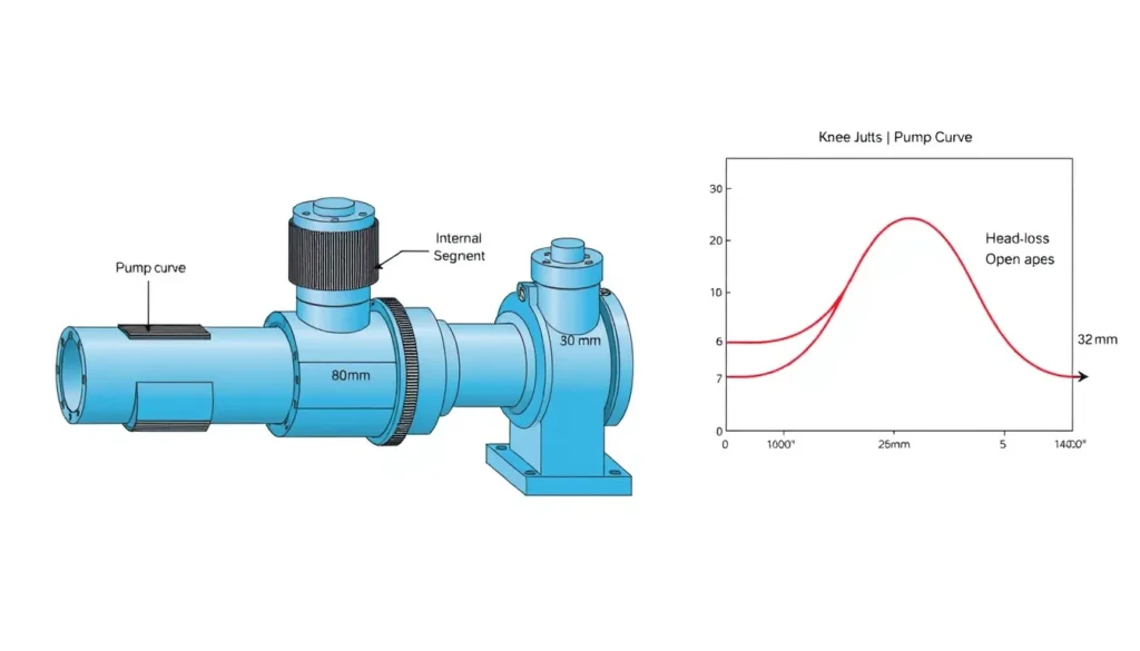
A system curve is a graphical or tabular relationship between the flow rate through a piping system and the total head required to deliver that flow. Building a system curve with multiple pipe diameters therefore requires segment-by-segment accounting whenever the system contains more than one pipe diameter—because of a header and smaller branches, a reducer, a manifold, or a series of sizes—there is no single pipe diameter that can be used in one friction equation. The curve must be built segment by segment, with continuity and common-node pressures enforced. The result is often not a simple parabola; it can have knees where a branch begins to flow or where flow regime changes.
Engineering relevance is high because the operating point is the intersection of the pump curve and the system curve. If the system curve is built with a wrong diameter or a lumped friction factor, the predicted flow and head can be off by a large margin. That error propagates into pump selection, motor sizing, control-valve authority, energy use, and reliability. In multi-diameter systems the most common failure is not the friction equation itself but the bookkeeping: flows in headers and branches, internal diameters, minor losses, and static heads must all be assigned to the correct segment.
This article uses the common encyclopedic scope: incompressible liquid flow in a pumped piping network with fixed geometry. It covers series sizes, parallel branches, and mixed networks. It does not attempt transient analysis or compressible-gas piping.
The Method — Derivation and Variants
Start from the steady-flow energy equation between the supply surface and the destination surface. For an incompressible fluid, total head required from the pump is the static head plus all losses between those points. The static part is Δz + (pd − ps)/(ρg). The loss part is the sum of major (pipe friction) and minor (fittings, valves, bends, area changes, exits) losses. For segment i with its own diameter Di and flow Qi, continuity gives vi = 4Qi/(πDi2). Darcy-Weisbach gives hf,i = fi(Li/Di)vi2/(2g). Minor loss is hm,i = ΣKivi2/(2g). Sum these over all segments that carry flow for the path being evaluated.
For series sizes, the same Q passes through every segment, so the segment losses simply add at that Q. For parallel branches, each branch sees a common node head Hn, but the branch flows differ. The node balance is Hn = zi + pi/(ρg) + lossesi(Qi) and Qtotal = ΣQi. If the branch flows are not controlled, solve this system iteratively or by a direct solve on Hn. If the branch flows are fixed by control valves or demand, a common shortcut is to compute each path from the source to its endpoint and take the greater required head; the lower-head branch then needs throttling to absorb the difference.
US customary and SI forms. The physics is identical; only the constants and unit conversions change. In US units, a convenient velocity form is v (ft/s) = 0.4085 Q (gpm)/D (in)2, and hf (ft) = f(L/D)v2/(2g) with L and D in ft and g = 32.2 ft/s2. In SI, v (m/s) = 4Q (m3/s)/(πD2), and hf (m) = f(L/D)v2/(2g) with g = 9.81 m/s2. Pressure head is H = 2.31 p (psi)/SG in US units and H = 0.102 p (kPa)/SG in SI, where SG is specific gravity. For water at standard conditions SG ≈ 1.0.
Friction factor f can be obtained from the Colebrook-White equation or the Moody chart. For water-only preliminary work, Hazen-Williams is an alternative: in SI, hf = 10.67 L Q1.852/(C1.852D4.87); in US customary, hf = 4.52 L Q1.852/(C1.852D4.87) with Q in gpm, D in inches, L in ft, and hf in ft. Hazen-Williams is less general than Darcy-Weisbach because it is tied to water and a roughness coefficient; Darcy-Weisbach is preferred when viscosity, temperature, or non-water fluids matter.
Equivalent-pipe variant. For a series of different diameters in turbulent flow, a segment can be converted to an equivalent length of a reference diameter: Leq = Lactual(Dref/Di)5. The exponent is 5 in turbulent flow and 4 in laminar flow. Use the diameter that gives the highest pressure drop as the reference to minimize error. This is a convenient check, not a substitute for a segment-by-segment branch balance.
Worked Example
Example 1 — SI branch network with an 80 mm header and two smaller branches. Water at 20°C (ρ = 998 kg/m3, μ = 0.001 Pa·s) is pumped through 50 m of 80 mm internal-diameter header (ε = 0.15 mm, minor K = 1.5). At the node it splits into Branch A: 30 m of 25 mm ID to an open tank 10 m above the pump, QA = 2 L/s = 0.002 m3/s, minor K = 2.5; and Branch B: 40 m of 32 mm ID to a sprinkler 5 m above the pump requiring 2 bar gauge, QB = 3 L/s = 0.003 m3/s, minor K = 1.5. Build the required pump head at total Q = 5 L/s.
Header: v1 = 4(0.005)/(π(0.080)2) = 0.995 m/s. Re1 = 998(0.995)(0.080)/0.001 = 7.94 × 10⁴. With ε/D = 0.001875, Swamee-Jain gives f1 ≈ 0.0254. Velocity head = v12/(2g) = 0.0505 m. Major loss = 0.0254(50/0.080)(0.0505) = 0.802 m. Minor loss = 1.5(0.0505) = 0.076 m. Header loss = 0.878 m.
Branch A: v2 = 4(0.002)/(π(0.025)2) = 4.07 m/s. Re2 ≈ 1.02 × 10⁵, ε/D = 0.006, f2 ≈ 0.0332. Velocity head = 0.844 m. Major loss = 0.0332(30/0.025)(0.844) = 33.6 m. Minor loss = 2.5(0.844) = 2.11 m. Branch A loss = 35.7 m. Required node head for A = 10 + 35.7 = 45.7 m.
Branch B: v3 = 4(0.003)/(π(0.032)2) = 3.73 m/s. Re3 ≈ 1.19 × 10⁵, ε/D = 0.00469, f3 ≈ 0.0308. Velocity head = 0.709 m. Major loss = 0.0308(40/0.032)(0.709) = 27.3 m. Minor loss = 1.5(0.709) = 1.06 m. Branch B loss = 28.4 m. Nozzle pressure head = 2 bar × 105/(998 × 9.81) = 20.4 m. Required node head for B = 5 + 20.4 + 28.4 = 53.8 m.
Take the greater branch requirement, Hnode = 53.8 m. Pump head at Q = 5 L/s is Hpump = Hnode + header loss = 53.8 + 0.878 = 54.7 m. Branch A would see 53.8 m at the node but needs only 45.7 m at its design flow, so a control valve or orifice must absorb about 8.1 m if QA is to remain 2 L/s. This is the controlled-flow shortcut; an uncontrolled open branch would take more flow and shift the operating point.
Example 2 — US customary series sizes. Water at 60°F flows at 200 gpm through 100 ft of 4-in Schedule 40 pipe (ID 4.026 in) then 150 ft of 6-in Schedule 40 pipe (ID 6.065 in), with a 20 ft elevation rise and minor losses: entrance K = 0.5, reducer K = 0.3 (on the smaller velocity), exit K = 1.0. v1 = 0.4085(200)/(4.026)2 = 5.04 ft/s; v2 = 0.4085(200)/(6.065)2 = 2.22 ft/s. Re1 ≈ 1.4 × 10⁵ and Re2 ≈ 9.3 × 10⁴; with ε = 0.00015 ft, f1 ≈ 0.0194 and f2 ≈ 0.0197. Velocity heads are 0.394 ft and 0.0766 ft. Major losses: 0.0194(100/0.3355)(0.394) = 2.28 ft and 0.0197(150/0.5054)(0.0766) = 0.448 ft. Minor losses: 0.5(0.394) + 0.3(0.394) + 1.0(0.0766) = 0.392 ft. Total head at 200 gpm = 20 + 2.28 + 0.448 + 0.392 = 23.1 ft. A first approximation of the curve is H ≈ 20 + 7.8 × 10⁻⁵ Q2 with Q in gpm and H in ft.
Calculator
For a single-path total dynamic head check, use this online Total Dynamic Head Calculator. For multi-branch or multi-diameter networks, use the calculator for each segment and then combine results with the node-balance method above, or use a pipe-network solver.
Reference Values & Typical Ranges
The following values are for preliminary water-system checks and should be replaced by project-specific data where available. Sources: HI Data Tool (system curves and head-loss fundamentals), Crane TP410 (minor losses and fluid flow), Karassik et al. Pump Handbook (branch-line pumping), and Modern Pumping Today (multi-branch system curves).
| Item | Typical range or rule of thumb | Engineering note |
|---|---|---|
| Suction-line velocity | 1–2 m/s (3–7 ft/s) | Lower velocities reduce NPSH risk and settling. |
| Discharge-line velocity | 2–3 m/s (6–10 ft/s) | Higher velocities increase friction and erosion. |
| Turbulent Darcy friction factor | 0.015–0.030 | Depends on Re and relative roughness; do not reuse across diameters. |
| Absolute roughness, new steel | ≈0.045 mm (0.00015 ft) | Age, fouling, and coatings can increase it. |
| 90° elbow minor K | ≈0.9 | Values vary with radius and manufacturer data. |
| Gate valve minor K | ≈0.2 fully open | Partially closed valves can dominate the system curve. |
| System-curve exponent | ≈2 for turbulent friction | Static-dominated curves are flatter; branch knees break the parabola. |
| Equivalent-pipe exponent | 5 turbulent; 4 laminar | Use the highest-loss diameter as the reference. |
Application Guidance
In real systems, the shape of the system curve drives pump selection more than any single number. A static-dominated curve—high elevation or pressure head and modest friction—is relatively flat, so small pump-head changes produce large flow changes. A friction-dominated curve is steeper, so added parallel pump capacity may yield diminishing flow increases. When multiple diameters are present, the curve often has a knee at the head where a low-static branch starts to flow. That knee is a hydraulic signature: below it, only one branch runs; above it, the second branch opens and the effective resistance changes.
For selection, generate the curve at the pump location, not only at a branch point. The pump sees the header loss plus the node head required by the worst-case branch. Check the intersection against the pump’s preferred operating region (POR), typically 70–120% of best efficiency point (BEP) for many ANSI/API pumps, with narrower ranges for some specific speeds under ANSI/HI 9.6.3. If the operating point moves outside the POR when a branch opens, consider a control valve, a variable-speed drive, or a different impeller trim.
Field judgment matters. Use actual internal diameters and actual lengths, including equivalent lengths for fittings. Add fouling margin on the friction term rather than on static head. For open-ended branches, remember that the branch with the least back pressure will take more flow unless it is throttled. If the branch discharges into a tank, include the exit loss; if it discharges to atmosphere, include the outlet velocity head. Confirm assumptions with a site sketch and a node-by-node flow balance before plotting the curve.
Common Mistakes, Limits & Safety Notes
- Using nominal size instead of internal diameter. Schedule, liner, and fouling change the ID; head loss scales roughly with D−5 in turbulent flow, so a small diameter error becomes a large head error.
- Reusing one friction factor or one K value for all diameters. Each segment has its own Reynolds number, relative roughness, velocity, and fittings.
- Adding branch flows without a common-node check. Parallel branches share one node head; they do not necessarily split in proportion to area or design flow.
- Treating an open-ended branch as fixed flow. An uncontrolled branch will seek its own operating point and can starve other users.
- Mixing US and SI units. Common errors include gpm with m3/h, psi with bar, and inches with millimetres in the same equation.
- Omitting minor losses at reducers, tees, exits, and valves. In short, multi-diameter runs these can exceed straight-pipe friction.
- Forgetting static head and pressure head. A friction-only curve cannot predict the zero-flow head or the effect of discharging into a pressurized vessel.
- Forcing a single parabola. Branch knees and flow-regime changes make the true curve piecewise; a single K is valid only after the split is fixed.
- Ignoring safety consequences. Under-predicted head can overload the motor or trip the pump; over-predicted head can lead to throttling, cavitation, vibration, and seal damage. Verify relief protection and control-valve authority.
FAQ
How do I calculate a system curve when pipe diameters change?
Break the system into segments by diameter and flow. For each segment, compute velocity from continuity, find the friction factor at that Reynolds number and relative roughness, then add Darcy-Weisbach friction and minor losses. For series sizes, add losses at the same flow. For branches, enforce a common node head and sum the branch flows.
Can I replace several pipe diameters with one equivalent pipe?
Yes for a series path in turbulent flow, using an equivalent length L_eq = L(D_ref/D)^5. Choose the highest-loss diameter as the reference. The method is a check and is not suitable for parallel branches whose split depends on a common node head. Recalculate the actual segments if the answer is critical.
What is the difference between series and parallel multi-diameter piping?
In series, the same flow passes through every diameter, so losses add directly. In parallel, each branch sees the same node head but carries a different flow. Series problems are straightforward substitutions; parallel problems require a node balance or iteration because the flow split is unknown until the branch resistances match.
How do I handle branches with different static heads?
Start at the lowest static-head branch. As node head rises, branches open in order of static head. Below a branch's static head it carries zero flow. Above it, use the branch loss equation to find flow. Sum flows at each node head to build the total system curve; the result is piecewise, not a single parabola.
What if one branch is open-ended and has almost no back pressure?
An open-ended branch will take more flow than a controlled branch unless it is throttled. Model it with the node balance, including exit loss and outlet velocity head. If you need a fixed design flow, add a control valve or orifice and check that it can absorb the excess head without cavitation or noise.
Should I use Darcy-Weisbach or Hazen-Williams?
Use Darcy-Weisbach when viscosity, temperature, non-water fluids, or accuracy across a wide Reynolds-number range matter. Hazen-Williams is acceptable for preliminary water-only checks at ordinary temperatures. For multi-diameter systems, either method must be applied segment by segment; do not use one lumped coefficient for all diameters.
How many points do I need for a system curve?
At minimum, calculate zero flow, the normal operating flow, and a flow above and below normal. For multi-branch systems, add points around each branch-opening head and around control-valve transitions. A smooth plot through 8–12 well-chosen points is usually enough for pump selection, but the knee points must be explicit.
Why is my system curve not a parabola?
A single parabola assumes one fixed resistance and fully turbulent flow. Multiple diameters, branch opening, laminar-to-turbulent transitions, control valves, and changing static heads all change the effective resistance. The true curve is piecewise; each segment may follow a Q-squared trend, but the combined curve can have knees and slope changes.
What units should I use for flow and diameter?
Use consistent units. In SI, Q in m³/s and D in m for v = 4Q/(πD²); or Q in L/s with a conversion. In US customary, Q in gpm and D in inches for v = 0.4085Q/D². Convert pressure to head with H = 2.31p/SG in US units or H = 0.102p/SG in SI.
How do I check if a pump is oversized for a multi-diameter system?
Plot the pump curve over the system curve at all expected branch conditions. If the intersection is far to the right of the best efficiency point or outside the preferred operating region, the pump may be oversized. Check motor power, control-valve authority, and whether throttling or variable speed can bring operation back toward BEP.

Leave a Reply