Short Answer
Key Formula / Key Facts Box
Governing Equation
[Delta P = K frac{rho V^{2}}{2}]
Where (Delta P) is the pressure drop (Pa or psi), (K) is the dimensionless loss coefficient, (rho) is fluid density (kg/m³ or lb/ft³), and (V) is the average flow velocity (m/s or ft/s).
| Symbol | Meaning | US Unit | SI Unit |
|---|---|---|---|
| ΔP | Pressure drop across the fitting | psi | Pa |
| K | Loss coefficient (dimensionless) | – | – |
| ρ | Fluid density | lb/ft³ | kg/m³ |
| V | Average flow velocity | ft/s | m/s |
Plain‑English: The pressure loss equals the K‑factor multiplied by the kinetic‑energy pressure of the fluid.
Overview — What It Is and Why It Matters
The K‑Factor table for valves and fittings is a compiled set of loss coefficients that characterize how much head (or pressure) a fluid loses when it negotiates a specific component. These coefficients are derived from experimental data or CFD analysis and are independent of pipe size; they capture geometry, turbulence, and flow‑direction effects.
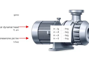
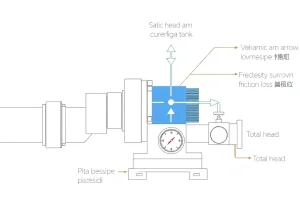
In hydraulic design, the total dynamic head supplied by a pump must overcome not only the static elevation but also the cumulative pressure drops of every fitting, valve, and pipe segment. An under‑estimated K‑value leads to inadequate pump sizing, cavitation, or excessive energy consumption, while an over‑estimated value inflates capital cost and may cause oversizing of equipment.
The Method — Derivation and Variants
Starting from the Bernoulli equation with an added head‑loss term, the pressure loss across a fitting is expressed as:
[frac{P_1}{rho g}+frac{V_1^{2}}{2g}+z_1 = frac{P_2}{rho g}+frac{V_2^{2}}{2g}+z_2 + h_L]
For a fitting the elevation change (z) is negligible and the velocity before and after is essentially equal (if the fitting does not change pipe diameter). The head loss (h_L) can be written as:
[h_L = K frac{V^{2}}{2g}]
Multiplying both sides by (rho g) converts head loss to pressure loss, yielding the key formula above.
Two common variants exist:
- US‑customary form: (Delta P_{psi}=Kfrac{rho_{lb/ft³} V_{ft/s}^{2}}{2}times 0.000145038) (conversion factor from psf to psi).
- SI form: (Delta P_{Pa}=Kfrac{rho_{kg/m³} V_{m/s}^{2}}{2}).
The constant 0.000145038 converts pounds‑force per square foot (psf) to pounds per square inch (psi). When dealing with incompressible liquids the density term is often combined with the velocity term to form the “dynamic pressure” (q=frac{rho V^{2}}{2}).
Worked Example
Example 1 – US Units (Water, 100 °F)
Given:
- Pipe Ø 2 in., schedule 40 (ID ≈ 2.067 in.)
- Flow rate Q = 400 gpm
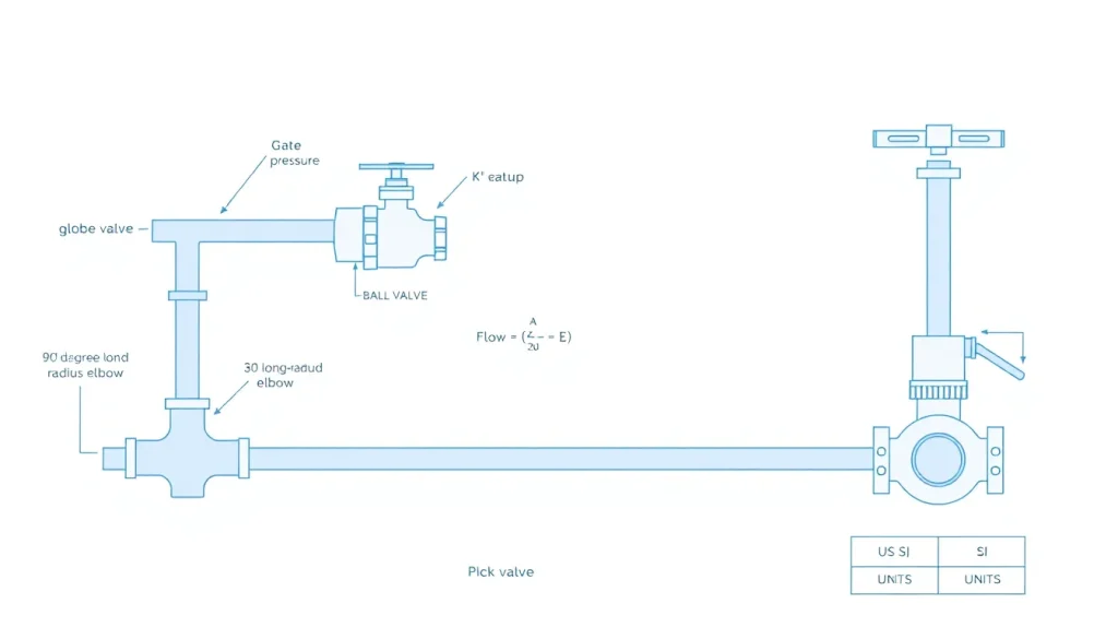
- Valve: globe valve, fully open, K = 10 (typical from table)
- Fluid density ρ = 62.4 lb/ft³ (water at 100 °F)
Step 1 – Convert flow to ft³/s:
[Q = 400,text{gpm}=frac{400}{7.4805},text{ft³/min}=53.5,text{ft³/min}=0.892,text{ft³/s}]
Step 2 – Calculate velocity:
Cross‑sectional area A = (pi D^{2}/4 = pi (2.067/12)^{2}/4 = 0.0235,text{ft²})
[V = Q/A = 0.892/0.0235 = 37.9,text{ft/s}]
Step 3 – Compute dynamic pressure:
[q = frac{rho V^{2}}{2}=frac{62.4times 37.9^{2}}{2}=44,800,text{lb/ft²}]
Convert to psi (1 psi = 144 lb/ft²):
[q_{psi}=frac{44,800}{144}=311,text{psi}]
Step 4 – Apply K‑factor:
[Delta P = K times q_{psi}=10times 311=3,110,text{psi}]
Because the pressure drop is unrealistically high, the engineer checks the K value; a globe valve at 100 % open typically has K≈5. Using K=5 yields 1,555 psi, still large, indicating the flow rate is excessive for a 2‑in. line.
Example 2 – SI Units (Oil, 20 °C)
- Pipe Ø 50 mm (ID ≈ 45 mm)
- Flow rate Q = 0.02 m³/s
- Fitting: 90° elbow, long radius, K = 0.30
- Fluid density ρ = 850 kg/m³
Step 1 – Area:
[A = frac{pi D^{2}}{4}=frac{pi (0.045)^{2}}{4}=1.59times10^{-3},text{m²}]
Step 2 – Velocity:
[V = Q/A = 0.02/1.59times10^{-3}=12.6,text{m/s}]
Step 3 – Dynamic pressure:
[q = frac{rho V^{2}}{2}=frac{850times 12.6^{2}}{2}=67,500,text{Pa}=0.675,text{bar}]
Step 4 – Pressure drop:
[Delta P = K times q = 0.30 times 67,500 = 20,250,text{Pa}=0.2025,text{bar}]
The elbow contributes only 0.20 bar of loss, a modest amount compared with pipe friction.
Calculator
For quick computations, use an online dynamic‑head calculator: PumpCalcs – Total Dynamic Head Calculator.
Reference Values & Typical Ranges
| Component | Typical K‑Range (US) | Typical K‑Range (SI) | Source |
|---|---|---|---|
| Gate valve – fully open | 0.15 – 0.35 | 0.15 – 0.35 | ASME B16.34 |
| Globe valve – 50 % open | 5 – 15 | 5 – 15 | ISA‑MFC‑3.0 |
| 90° elbow, short radius | 0.90 – 1.30 | 0.90 – 1.30 | API 650 |
| 90° elbow, long radius | 0.30 – 0.50 | 0.30 – 0.50 | API 650 |
| Ball valve – fully open | 0.05 – 0.15 | 0.05 – 0.15 | ISO 5752‑2 |
| Check valve – free flow | 0.5 – 2.0 | 0.5 – 2.0 | ASME B16.34 |
Note: Values are for incompressible liquids at Reynolds numbers >10⁴. Gases require compressible‑flow corrections.
Application Guidance
- Sum all K‑values for a loop and convert to head loss using the dynamic pressure at the design flow rate.
- When multiple fittings of the same type are present, multiply the K‑value by the quantity before adding to the total.
- For tapered or reduced‑diameter fittings, use the velocity based on the smaller diameter for the K‑calculation.
- In pump‑selection software, input the total equivalent length (L_eq = ΣK·D) to incorporate fitting losses into the friction‑loss calculation.
- For high‑viscosity fluids, consult manufacturer‑provided K‑corrections; the standard table assumes Newtonian behavior.
Common Mistakes, Limits & Safety Notes
- Unit mismatch: Using ρ in kg/m³ with V in ft/s produces nonsensical results. Always keep US units together or SI units together.
- Applying K‑values at low Reynolds numbers: The tabulated coefficients assume turbulent flow; laminar regimes reduce K dramatically.
- Ignoring pipe‑diameter effect on velocity: K itself is dimensionless, but the dynamic pressure depends on V, which changes with pipe size.
- Double‑counting losses: Do not add both K‑based loss and equivalent length loss for the same fitting.
- Using “fully open” K for partially throttled valves: Throttling can increase K by an order of magnitude.
- Neglecting temperature‑dependent density: For gases or heated liquids, density variations alter dynamic pressure significantly.
- Safety oversight: Under‑estimating total head can cause cavitation, pump overheating, or system over‑pressurization, jeopardizing personnel and equipment.
FAQ
How do I choose the correct K‑factor for a valve that is not fully open?
Select the K‑value that corresponds to the valve’s percent open or throttling position, which is usually provided in the manufacturer’s data sheet. If only full‑open data are available, apply a correction factor (often 5‑10×) based on empirical charts.
Can I use the same K‑table for gases as for liquids?
Standard K‑tables assume incompressible liquids. For gases, the density changes with pressure and temperature, so you must recompute the dynamic pressure term and often apply compressibility corrections or use gas‑specific K‑values.
Why does the K‑factor for a 90° elbow differ between short and long radius?
A long‑radius elbow allows the flow to change direction more gradually, reducing separation and turbulence, which lowers the loss coefficient compared with a sharp, short‑radius bend.
Is it acceptable to ignore minor losses in a large‑diameter pipe system?
Minor losses become insignificant only when the total fitting loss is less than 5 % of the friction loss. In high‑speed or low‑head systems, even a few fittings can dominate the total head.
How does fluid viscosity affect K‑values?
Viscosity has a minor effect for turbulent flow, but for laminar or transitional regimes the loss coefficient decreases with increasing viscosity. Manufacturers sometimes provide viscosity‑corrected K‑factors for heavy oils.
What safety factor should I apply to total head calculations?
A common practice is to add 10‑15 % margin to the calculated total dynamic head to accommodate future flow increases, fouling, and measurement uncertainties.
Do I need to convert K‑values when switching between US and SI units?
No. K is dimensionless, so the same numeric value applies regardless of unit system; only the surrounding terms (ρ, V, ΔP) require unit consistency.
How do I account for a series of identical fittings?
Multiply the single‑fitting K‑value by the number of occurrences before adding it to the system loss sum. For example, three identical elbows: K_total = 3 × K_elbow.
What is the impact of pipe roughness on K‑values?
Pipe roughness influences friction loss, not the K‑value of fittings. However, roughness can indirectly affect the local flow pattern and slightly modify K, especially for low‑Re flows.
Can I use CFD to generate my own K‑tables?
Yes. CFD simulations calibrated with experimental data can produce component‑specific loss coefficients, which is useful for custom or non‑standard fittings.
Leave a Reply