
Short Answer
Key Formula / Key Facts Box
Governing system relationship: H = Hst + k Q2
Actual power ratio for a fixed system: P2/P1 = (Q2/Q1) × (Hst + k Q22) / (Hst + k Q12)
Cube-law shortcut, valid only when Hst ≈ 0: P2/P1 ≈ (Q2/Q1)3
| Symbol | Meaning | US unit | SI unit |
|---|---|---|---|
| P | Pump shaft or brake power | hp | kW |
| Q | Volumetric flow rate | gpm | m3/s |
| H | Total system head | ft | m |
| Hst | Static head, independent of flow | ft | m |
| k | Friction coefficient, Hf = k Q2 | ft/gpm2 | m/(m3/s)2 |
| η | Pump or pump-motor efficiency | dimensionless | dimensionless |
Plain-English restatement: The cubic shortcut assumes every unit of head disappears as flow falls; in a high-static-head system, most of the head is still there, so power falls much less than flow cubed.

Overview — What It Is and Why It Matters
This article uses the common encyclopedic meaning of the cube law in pump engineering: the affinity-law shortcut that pump power varies with the cube of flow, P ∝ Q³, or with the cube of speed, P ∝ N³, when a centrifugal pump operates along a system curve that passes through the origin. The scope is VFD-controlled centrifugal pumps in open or high-static-head systems where Hst is a large fraction of total head. In such systems, the cube law overestimates VFD savings because static head does not shrink with flow.
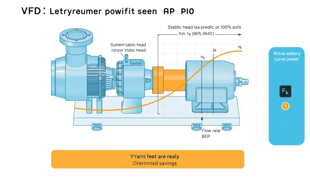
Static head comes from elevation differences, tank levels, well depth, fixed discharge pressure, or minimum pressure controls. Friction head comes from pipe, fittings, valves, and heat exchangers and varies roughly with flow squared. A closed-loop system with no static head has a system curve through the origin, and the cube law works well. An open system with high static head has a system curve that starts at a positive head on the y-axis. When flow is reduced, the pump still must overcome that positive head, so power cannot fall as fast as Q³.
The consequence of the error is practical: predicted payback periods become too short, energy-savings contracts may underdeliver, and in some open systems a VFD can use more energy than well-designed on/off control. The ACEEE study by Jones and Barrer notes that in open systems with significant static head, savings can be much less than shortcut affinity-law estimates and occasionally negative. Maxwell lists independent head elements, less-than-square head changes, minimum static pressure controls, efficiency changes, motor part-load efficiency, drive losses, and measured full-flow power as common sources of overestimation.
The Method — Derivation and Variants
Hydraulic power is Ph = ρ g Q H. With efficiency η, brake power is P = ρ g Q H / η. For a fixed system, H = Hst + k Q². Substituting gives P = ρ g Q (Hst + k Q²) / η. Taking the ratio at two flows cancels ρ, g, and η if efficiency is constant. The result is the actual power ratio shown in the key box. When Hst = 0, H1 = k Q1², so P2/P1 = (Q2/Q1) × (k Q2²)/(k Q1²) = (Q2/Q1)³. This is the only condition in which the cubic flow shortcut is exact for a fixed system curve.
| Form | Equation |
|---|---|
| US customary | BHP = Q(gpm) × H(ft) × SG / (3960 × η) |
| SI | P(kW) = ρ(kg/m³) × 9.81 × Q(m³/s) × H(m) / (1000 × η) |
The constant 3960 combines unit conversions and water density at standard conditions; for fluids with SG ≠ 1, multiply by SG. The SI form uses ρ explicitly. The dimensionless power ratio is identical in both systems.
Speed variant: The affinity laws Q ∝ N, H ∝ N², and P ∝ N³ describe geometrically similar operating points. In a high-static-head system, reducing flow moves the operating point to a different affinity parabola, so P₂/P₁ = (N₂/N₁)³ is not valid between the original and new system points. The speed reduction needed to reach a given flow is also limited: the pump must still generate at least Hst. A useful approximation for a pump curve represented by Hp = H₀ − aQ² and a system H = Hst + bQ² is s² = (Hst + (a+b)Q₂²)/(Hst + (a+b)Q₁²), where s = N₂/N₁. This shows that s remains much closer to 1 than Q₂/Q₁ when static head dominates.
Worked Example
US customary example. A transfer pump runs at Q₁ = 1,000 gpm and H₁ = 200 ft. Static head is Hst = 150 ft, so design friction head is 50 ft. Efficiency is assumed 75% and SG = 1.0. Full-flow brake power is BHP₁ = 1,000 × 200 / (3,960 × 0.75) = 67.3 hp. The friction coefficient is k = 50 / 1,000² = 5.0 × 10⁻⁵ ft/gpm². At Q₂ = 500 gpm, friction head is kQ₂² = 5.0 × 10⁻⁵ × 500² = 12.5 ft, and total head is H₂ = 150 + 12.5 = 162.5 ft. Actual power is BHP₂ = 500 × 162.5 / (3,960 × 0.75) = 27.4 hp. The actual power ratio is 27.4/67.3 = 0.406, or 40.6%. The cube law predicts (500/1,000)³ = 0.125, or 8.4 hp. The shortcut predicts 58.9 hp of savings; the actual saving is 39.9 hp, so the cube law overestimates savings by about 19.0 hp, or 47% of the actual saving. If the pump shutoff head is 250 ft, the required speed ratio is s² = (150 + 1.0×10⁻⁴×500²)/(150 + 1.0×10⁻⁴×1,000²) = 0.70, so s = 83.7%, not 50%.
SI example. The same case is Q₁ = 0.0631 m³/s, H₁ = 61.0 m, Hst = 45.7 m, friction = 15.2 m, η = 0.75, and ρ = 1,000 kg/m³. Full-flow power is P₁ = 1,000 × 9.81 × 0.0631 × 61.0 / (1,000 × 0.75) = 50.3 kW. The friction coefficient is k = 15.2 / 0.0631² = 3,820 m/(m³/s)². At Q₂ = 0.03155 m³/s, friction head is 3,820 × 0.03155² = 3.80 m, and H₂ = 45.7 + 3.80 = 49.5 m. Actual power is P₂ = 1,000 × 9.81 × 0.03155 × 49.5 / (1,000 × 0.75) = 20.4 kW. The actual ratio is 20.4/50.3 = 0.406. The cube law predicts 0.125 × 50.3 = 6.29 kW. Again, the cube law understates power at the reduced flow and overstates VFD savings.
Calculator
Use a total dynamic head calculator such as pumpcalcs.com total dynamic head calculator to separate static and friction head before estimating VFD savings.
Reference Values & Typical Ranges
The table shows how the actual power ratio varies with static head fraction when flow is halved. It uses the system formula with constant efficiency.
| Static head fraction Hst/H₁ | Actual P₂/P₁ at Q₂/Q₁ = 0.50 | Cube-law P₂/P₁ | Savings overestimate from cube law |
|---|---|---|---|
| 0.00 | 0.125 | 0.125 | None |
| 0.25 | 0.219 | 0.125 | 9.4 percentage points |
| 0.50 | 0.313 | 0.125 | 18.8 percentage points |
| 0.75 | 0.406 | 0.125 | 28.1 percentage points |
| 1.00 | 0.500 | 0.125 | 37.5 percentage points |
Rules of thumb from the literature:
- Closed-loop, friction-only systems have Hst ≈ 0 and closely follow P ∝ Q³; open systems with tanks, wells, or fixed discharge pressure do not [1][2].
- In open systems with significant static head, VFD savings can be much less than shortcut affinity-law estimates, and VFDs may use more energy than on/off control in some cases [1].
- High static head factor fHS = Hst/H₁ is a key screen; Martins and Lima note that even fHS as high as 80% can still justify VFD for reliability and control, but energy gains are reduced and unstable pumpage risk rises [5].
- Pump efficiency at the new operating point can be up to 5.4% lower than at design in the ORNL example; do not assume constant efficiency for final savings estimates [3].
- Maxwell lists independent head elements, less-than-square head changes, minimum static pressure controls, efficiency changes, motor part-load efficiency, drive losses, and measured full-flow power as common sources of overestimation [2].
- Throttling versus VFD: VFDs often save versus throttling even with static head, but the comparison must be against the actual existing control, not against an ideal friction-only curve [4].
Application Guidance
Start by measuring or estimating the system curve. Separate static head—tank elevation, well depth, fixed discharge pressure, and minimum pressure controls—from friction and minor losses. If static head is more than about 50% of design head, treat cube-law estimates as an upper bound, not a prediction. Calculate power at each turndown point using P = ρgQH/η, and use the pump curve at the required speed rather than assuming Q₂/Q₁ = N₂/N₁. Check that the pump can meet Hst at the minimum speed and that flow remains above minimum continuous stable flow. In level-control systems, compare VFD operation with efficient on/off control; on/off operation often runs near BEP and may be more efficient when the tank provides storage. VFDs may still be justified for soft starts, pressure stability, reliability, reduced throttling losses, and avoidance of recirculation, even when energy savings are modest. For high-static-head systems, verify motor and drive losses at part load, pump efficiency at the new operating point, NPSH margin, seal and bearing life, and any minimum-flow bypass. Field adjustments include using actual valve positions, tank levels, and pressure setpoints to build the real system curve rather than a design-office approximation.
Common Mistakes, Limits & Safety Notes
- Applying P₂/P₁ = (Q₂/Q₁)³ to a system curve that does not pass through the origin. This is the central error; it assumes static head is zero.
- Confusing flow ratio with speed ratio. In high-static-head systems, a 50% flow reduction may require 80–90% speed, not 50% speed.
- Ignoring static head or misclassifying it as friction. Use Hst = discharge elevation/pressure minus suction elevation/pressure, independent of flow.
- Using nameplate power as the baseline. Measure full-flow input power; nameplate and design power can differ substantially [2].
- Assuming constant pump efficiency. Efficiency can drop at reduced speed and flow, especially below about 66.7% speed; use the pump curve or ORNL-style correction [3].
- Forgetting motor and VFD losses at part load. Small motors below about 35% load may have lower efficiency, and drive losses must be included [2].
- Ignoring minimum speed and minimum continuous stable flow. The pump may not overcome static head or may operate in an unstable, recirculating region.
- Assuming a VFD always beats on/off control. In some open systems, on/off control is more efficient and a VFD can increase energy use [1].
- Neglecting control valves, bypasses, and minimum pressure controls. These elements can change the system curve and invalidate a simple quadratic model.
- Safety consequence: low-flow operation can cause overheating, cavitation, seal damage, and vibration. Verify NPSH margin, pressure relief, fail-safe speed, and MCSF before commissioning.
FAQ
Why does the cube law overestimate VFD savings in my high-static-head pump system?
The cube law assumes the system curve passes through the origin, so all head falls as flow falls. In a high-static-head system, much of the head remains even at low flow, so power stays higher than Q³ predicts. The pump also cannot reduce speed as much because it must still overcome static head.
How can I tell if my system has high static head?
Measure head at zero or very low flow and compare it with design head. If the pump still produces substantial pressure with no flow, that is static head. Open systems with tanks, wells, or fixed discharge pressure often have static head fractions of 50–80%.
Can a VFD actually increase energy use in a high-static-head system?
Yes. In some open systems, especially those previously controlled on/off, a VFD may run the pump for longer periods at reduced speed and can use more energy than efficient on/off control. The ACEEE study found cases where VFDs were not cost-effective and occasionally used more energy.
What is the difference between static head and friction head for VFD savings?
Static head is independent of flow and does not disappear when the pump slows. Friction head varies roughly with flow squared and falls at lower flow. VFD savings are largest when friction dominates and smallest when static head dominates.
How do I calculate actual VFD savings with static head?
Use P = ρgQH/η at the original and new operating points, with H = H_st + kQ². Measure or estimate static head, friction coefficient, and efficiency. Do not use P₂/P₁ = (Q₂/Q₁)³ unless static head is negligible.
What minimum speed can my pump run at with high static head?
The minimum speed must produce enough head to overcome static head and maintain stable flow. It depends on the pump curve and system. Check the pump curve at reduced speed and verify operation above minimum continuous stable flow; otherwise the pump may stall or recirculate.
Does pump efficiency change when a VFD reduces speed?
Yes. Efficiency often stays close to design at moderate speed reduction, but it can drop at low speed and low flow. ORNL reports up to 5.4% lower efficiency at new operating points in one example, so use the pump curve or a correction method for final estimates.
Are VFDs still worthwhile on high-static-head systems?
Often yes, but the justification may be reliability, pressure control, soft starting, reduced throttling, or avoidance of recirculation rather than large energy savings. Compare against the actual existing control and verify payback with realistic power calculations.
How does on/off control compare with VFD control in high-static systems?
On/off control often runs the pump near its best efficiency point when operating and may be more efficient than continuous VFD operation in some level-control systems. VFDs can still help where frequent starts, pressure swings, or throttling losses are problems.
What standards or guides cover pump system energy assessment?
Useful references include US DOE pump system assessment guidance, ASME pump standards, ISO 9906 for pump performance testing, and ORNL/ACEEE energy-efficiency methods. The key is to use the actual system curve and measured power rather than a cube-law shortcut.

Leave a Reply