Short Answer
Why the Motor Matters More Than the Pump
It is tempting to treat the motor as an afterthought—size the pump, then bolt on whatever motor produces enough horsepower. This is backward. The Hydraulic Institute’s life cycle cost studies consistently show that for a pump operating continuously or near-continuously, energy cost dwarfs every other cost category, typically representing 85–90% of the total cost of ownership over a 15–20 year service life. Purchase price, installation, and even maintenance are comparatively minor.
That energy cost is determined almost entirely by three decisions made at the motor and drive level:
- Motor efficiency class — a 2–4 percentage-point efficiency difference, sustained over tens of thousands of running hours, is real money.
- Whether the pump runs at fixed speed or variable speed — a VFD matched to a variable-demand system can cut energy consumption by 30–50% or more.
- Correct sizing — an oversized motor running at partial load operates less efficiently and costs more up front; an undersized motor overheats and fails.
This pillar covers all three, plus the starting methods and electrical sizing calculations that determine whether the motor and drive will actually work reliably in your system.
Motor Sizing Fundamentals
From Brake Power to Motor Power
The pump’s brake horsepower (BHP) is the mechanical power required at the pump shaft, calculated from flow, head, specific gravity, and pump efficiency (see the Pump Hydraulics pillar for the full derivation):
$$P_{\text{brake}} \text{ (HP)} = \frac{Q \text{(gpm)} \times H \text{(ft)} \times \text{SG}}{3960 \times \eta_{\text{pump}}}$$
The motor power required is the brake power divided by motor efficiency, then multiplied up for a safety margin:
$$P_{\text{motor}} = \frac{P_{\text{brake}}}{\eta_{\text{motor}}} \times SF_{\text{design}}$$
where $SF_{\text{design}}$ is a design margin (distinct from the motor’s own nameplate service factor, discussed below)—typically 1.10–1.15 to account for pump curve tolerance, system uncertainty, and future conditions.
Service Factor: What It Actually Means
A motor’s nameplate service factor (SF) is the multiplier by which the motor can be safely overloaded above its rated horsepower, on a continuous basis, without exceeding its insulation temperature limits—provided voltage and frequency are at rated values. A motor rated 10 HP with SF 1.15 can sustain 11.5 HP continuously without immediately failing.
This is not the same thing as a design safety margin, and conflating the two is one of the most common sizing errors:
- Design margin is a decision you make: how much headroom to add for pump curve tolerance, future flow increases, or measurement uncertainty.
- Service factor is a property of the motor itself, intended as a reserve for unusual conditions (voltage sag, minor pump wear increasing torque, temporary overload)—not as routine operating margin.
Correct practice: size the motor so that your expected continuous brake power demand sits comfortably within 100% of the motor’s nameplate horsepower. The service factor exists as a buffer for abnormal conditions, not as your everyday design margin. Running a motor continuously into its service-factor zone shortens winding life and voids some manufacturer warranties.
Two Sizing Philosophies
| Philosophy | Approach | Trade-off |
|---|---|---|
| Non-overloading | Select a motor whose nameplate HP exceeds the maximum brake power anywhere on the pump curve (including runout conditions at the far right of the curve) | Larger, more expensive motor; guarantees the motor never depends on its service factor |
| Service-factor-assisted | Select a motor whose nameplate HP covers normal operation, relying on SF to cover runout or transient conditions | Smaller, cheaper motor; acceptable only if runout conditions are brief and infrequent |
For centrifugal pumps, always check the brake power at the runout point (the far-right end of the pump curve, at maximum flow / minimum head)—power typically continues rising with flow even as head drops, and runout is where many “correctly sized” motors actually overload.
Standard Motor Sizes: NEMA and IEC Ladders
Motors are manufactured in a discrete set of standard sizes. Once you calculate required motor power, you select the next standard size up—never a custom or interpolated value.
NEMA (US Customary) Horsepower Ladder
$$0.5,\ 0.75,\ 1,\ 1.5,\ 2,\ 3,\ 5,\ 7.5,\ 10,\ 15,\ 20,\ 25,\ 30,\ 40,\ 50,\ 60,\ 75,\ 100,\ 125,\ 150,\ 200,\ 250,\ 300\ (\text{HP})$$
IEC (Metric) Kilowatt Ladder
$$0.37,\ 0.55,\ 0.75,\ 1.1,\ 1.5,\ 2.2,\ 3,\ 4,\ 5.5,\ 7.5,\ 11,\ 15,\ 18.5,\ 22,\ 30,\ 37,\ 45,\ 55,\ 75,\ 90,\ 110,\ 132,\ 160\ (\text{kW})$$
Example: you calculate a required motor power of 57.6 HP with a 1.15 design margin applied, giving 66.2 HP. The next standard NEMA size is 75 HP—not 60 HP, which would leave no margin at all.
Motor Frame Sizes
Beyond horsepower, motors are built on standardized frame sizes (NEMA frame numbers like 143T, 145T, 182T, 213T, 254T, and so on) that fix the shaft height, shaft diameter, bolt pattern, and mounting dimensions. Two motors of the same horsepower can have different frame sizes depending on speed (a 1,800 RPM motor is typically a larger frame than a 3,600 RPM motor of the same HP, because more torque must be carried at lower speed). Always confirm frame size compatibility with the pump’s coupling or baseplate before ordering—a horsepower match alone does not guarantee a bolt-up fit.
Motor Efficiency Classes
The Efficiency Landscape
Electric motor efficiency is standardized into classes, and the classes in force have tightened substantially over the past two decades as energy codes have pushed the market toward higher efficiency.
| Class (IEC) | US equivalent | Typical description |
|---|---|---|
| IE1 | “Standard efficiency” | Legacy designs, largely phased out in most developed markets for new motors |
| IE2 | “EPAct” (Energy Policy Act baseline) | The pre-2010 US minimum standard |
| IE3 | “NEMA Premium” | The current mandated minimum for most general-purpose motors in the US (per EISA 2007/2010) and widely mandated internationally |
| IE4 | “Super premium” | Voluntary, higher-cost, higher-efficiency tier—typically justified only for very high running-hour applications |
For nearly all new pump motor purchases in the US today, IE3 / NEMA Premium is the practical baseline—it is what most manufacturers stock and what codes require for general-purpose induction motors in most horsepower ranges. IE4 is worth the incremental cost primarily for motors running continuously (8,000+ hours/year) where the efficiency gain compounds over a long service life.
The Efficiency Gap Is Small in Percentage, Large in Dollars
The difference between an IE2 and an IE3 motor might be only 2–3 efficiency percentage points (e.g., 91% vs. 93.5% for a 50 HP motor). That sounds trivial until you compute it over the motor’s service life:
- A 50 HP motor running 8,760 hours/year at $0.12/kWh
- At 91% efficiency vs. 93.5% efficiency, the input power differs by roughly 1.5 kW
- Annual cost difference: $0.12 \times 1.5 \times 8760 \approx $1,577/\text{year}$
- Over a 15-year service life: over $23,000
This is why efficiency class is not a minor spec line—for continuously running pumps, it is one of the largest economic levers available.
Efficiency Varies with Load
A motor’s nameplate efficiency is quoted at 100% rated load. Efficiency typically peaks near 75–100% of rated load and drops off at partial load (below ~50%)—another reason to avoid grossly oversizing a motor “just to be safe.” A motor running continuously at 30% load is both wasting the extra capital spent on motor size and operating at reduced efficiency.
Three-Phase vs. Single-Phase Motors
| Characteristic | Three-phase | Single-phase |
|---|---|---|
| Typical size range | 0.5 HP and up; standard above ~5 HP | Typically limited to ≤ 5–10 HP |
| Starting torque | Smooth, self-starting | Requires a starting mechanism (capacitor-start, split-phase) |
| Efficiency | Higher at equivalent HP | Lower, more losses |
| Vibration/noise | Smoother running | More pulsation, more vibration |
| Availability | Requires three-phase utility service or a phase converter/VFD | Standard residential service |
| Typical pump application | Commercial, industrial, most wells and boosters above residential scale | Small residential well pumps, small circulators, sump pumps |
Practical guidance: if three-phase power is available at the site, use it for anything above a few horsepower—efficiency, reliability, and smoothness all favor it. Where only single-phase utility service exists and the load exceeds what a single-phase motor comfortably handles, a VFD with single-phase input and three-phase output (a “phase converter” function built into many drives) is often more cost-effective than installing a dedicated rotary phase converter.
Motor Starting Methods
How a motor is brought up to speed matters for both the electrical system (inrush current, voltage sag) and the mechanical system (starting torque, water hammer from sudden flow onset).
Direct-On-Line (DOL) Starting
The motor is connected directly to full voltage. Simplest and cheapest, but draws the highest inrush current—typically 6–8× the motor’s full load amps (FLA) for 1–2 seconds.
- Best for: small motors (typically under 20–30 HP, depending on the utility’s tolerance for voltage sag) where the electrical system can absorb the inrush without disturbing other loads.
- Limitation: on weak electrical services, the voltage sag from DOL starting can dim lights, trip sensitive equipment, or exceed utility-imposed inrush limits.
Star-Delta (Wye-Delta) Starting
The motor windings are initially connected in “star” (wye) configuration for starting, which reduces starting current to roughly 1/3 of DOL, then switched to “delta” configuration for running at full torque and speed.
- Best for: medium motors (roughly 15–200 HP) where DOL inrush is unacceptable but a VFD is not justified.
- Limitation: the transition from star to delta causes a torque and current transient; for pump loads (which have relatively low starting torque requirements compared to, say, conveyors), this is usually acceptable, but it should not be used on loads sensitive to torque transients.
Soft Starters
A solid-state device that gradually ramps up voltage (and therefore torque and current) over a few seconds, rather than switching abruptly.
- Reduces inrush to roughly 2–4× FLA, smoother than star-delta with no transition transient.
- Best for: applications where gentle acceleration reduces water hammer risk (long discharge pipelines) or mechanical stress (belt-driven pumps, couplings).
- Limitation: does not provide ongoing speed control after starting—once ramped up, the motor runs at full line frequency.
Variable Frequency Drives (VFDs)
A VFD provides the smoothest possible start (current limited to as low as 1× FLA if desired) and ongoing speed control throughout operation. See the dedicated section below—VFDs are covered separately because their primary value proposition (energy savings) extends far beyond starting behavior.
Starting Method Comparison
| Method | Inrush current | Torque control | Ongoing speed control | Relative cost |
|---|---|---|---|---|
| DOL | 6–8× FLA | None | None | Lowest |
| Star-Delta | ~2–3× FLA | Limited (transition transient) | None | Low |
| Soft Starter | 2–4× FLA | Good (ramped) | None | Moderate |
| VFD | As low as 1× FLA | Excellent | Full range | Highest |
Variable Frequency Drives: How They Work and When They Save Energy
How a VFD Works
A VFD converts incoming fixed-frequency AC power (e.g., 60 Hz) to DC, then synthesizes a variable-frequency AC output that controls motor speed. Since induction motor speed is directly proportional to supply frequency, varying the frequency from, say, 30 Hz to 60 Hz varies motor speed from roughly 50% to 100% of nameplate RPM.
The Cube Law and Why VFDs Save Energy
Recall the pump affinity laws from the Pump Hydraulics:
$$\frac{Q_2}{Q_1} = \frac{N_2}{N_1} \qquad \frac{H_2}{H_1} = \left(\frac{N_2}{N_1}\right)^2 \qquad \frac{P_2}{P_1} = \left(\frac{N_2}{N_1}\right)^3$$
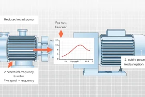
Power varies with the cube of speed. Reducing pump speed to 80% of full speed reduces power demand to roughly $0.8^3 = 0.512$, or about half the power, while flow drops only to 80%. This is why VFDs are so effective on variable-demand systems: a modest speed reduction produces a disproportionately large energy saving.
The Critical Caveat: Static Head Breaks the Cube Law
The cube law above assumes the system curve has zero static head—all resistance is friction. Most real systems have some static head component (elevation change, or a minimum discharge pressure requirement), and static head does not scale with speed. The system curve is:
$$H_{\text{system}} = H_{\text{static}} + K \times Q^2$$
The higher the proportion of static head relative to friction head, the less benefit a VFD provides, because a larger fraction of the pump’s work is fixed regardless of speed. In the extreme case of a system that is entirely static head (e.g., pumping to a fixed-elevation tank with negligible friction), reducing pump speed reduces flow but the pump still must produce at least the static head—drop speed too far and the pump simply cannot overcome the static head at all, and flow goes to zero abruptly rather than gracefully.
Practical implication: VFDs deliver the largest savings on systems dominated by friction losses and variable demand (HVAC circulation, irrigation with variable zones, process systems with fluctuating flow requirements). They deliver much smaller savings—sometimes none worth the investment—on systems dominated by static head with fairly constant demand (a well pump filling a fixed-elevation tank at a steady rate, for instance).
Always model the actual system curve, including its static head fraction, before promising VFD energy savings. A vendor quote based on the cube law alone, without checking the static head fraction, will overstate savings.
When a VFD Is the Wrong Choice
- Constant-speed, constant-demand applications with little static head don’t benefit much—the pump already runs near its optimum point continuously.
- High static head systems with modest friction see limited savings, as explained above.
- Positive displacement pumps generally don’t benefit from VFD speed control in the same way—flow is already nearly proportional to speed with PD pumps, but the pressure the system develops is set by resistance/relief, not by matching a parabolic system curve; the energy-saving mechanism that makes VFDs valuable on centrifugal pumps doesn’t translate the same way.
- Very low minimum flow requirements combined with high static head can push the pump below its minimum stable flow at low VFD speeds, risking recirculation and heat buildup—check the pump’s minimum flow curve before specifying a wide VFD turndown range.
Additional VFD Benefits Beyond Energy
- Reduced mechanical stress: soft ramp-up and ramp-down reduce water hammer and shock loading on piping, couplings, and bearings.
- Process control: VFDs allow closed-loop control (e.g., maintaining constant discharge pressure via a pressure transducer feedback signal) that fixed-speed pumps cannot achieve without external control valves.
- Multiple-pump staging: in systems with several parallel pumps, VFDs allow one pump to trim precisely to demand while others cycle on/off in fixed-speed steps, optimizing overall system efficiency.
Electrical Sizing: FLA, Voltage Drop, and Power Factor
Full Load Amps (FLA)
Full load amps is the current a motor draws at its rated horsepower, rated voltage, and rated frequency. For a three-phase motor:
$$I_{\text{FLA}} \text{(A)} = \frac{P \text{(HP)} \times 746}{\sqrt{3} \times V \times \eta_{\text{motor}} \times \text{PF}}$$
where $V$ is line-to-line voltage, $\eta_{\text{motor}}$ is motor efficiency, and PF is power factor.
Example: a 10 HP, 460V, three-phase motor with 90% efficiency and 0.85 power factor:
$$I_{\text{FLA}} = \frac{10 \times 746}{1.732 \times 460 \times 0.90 \times 0.85} = \frac{7460}{610.1} = 12.2 \text{ A}$$
Always verify FLA against the manufacturer’s nameplate rather than relying solely on calculation—actual motor design details cause nameplate FLA to vary somewhat from the theoretical formula.
Voltage Drop
Voltage drop in the supply cable reduces the voltage actually available at the motor terminals, which can cause overheating, reduced starting torque, and premature failure if excessive. A simplified voltage drop calculation for a single-phase or DC circuit:
$$VD \text{(V)} = \frac{2 \times L \times I \times R}{1000}$$
where $L$ is one-way cable length (ft), $I$ is current (A), and $R$ is cable resistance (ohms per 1,000 ft, from wire gauge tables). For three-phase circuits, a $\sqrt{3}$ factor replaces the 2.
Rule of thumb: keep voltage drop under 3% for branch circuits and under 5% total (feeder + branch) per NEC recommendations. Excessive voltage drop is especially common on long submersible pump drop-cable runs in deep wells—always size the cable for the run length, not just the current, and consult a voltage-drop table or the Voltage Drop Calculator.
Power Factor
Power factor (PF) is the ratio of real (working) power to apparent power, reflecting the phase difference between voltage and current caused by the motor’s inductive nature. Typical induction motor power factor ranges from 0.80 to 0.90 lagging at full load, dropping significantly at partial load (a lightly loaded motor might have PF as low as 0.5–0.6).
Why it matters: utilities often penalize industrial customers for poor power factor (below ~0.90–0.95, depending on the utility’s tariff), because low power factor increases current for the same real power delivered, straining the distribution system. Power factor correction capacitors, sized to offset the motor’s inductive reactance, can raise the effective power factor at the meter without changing the motor’s actual operation.
$$\text{Correction capacitor kVAR} = P_{\text{real (kW)}} \times (\tan\phi_1 – \tan\phi_2)$$
where $\phi_1$ and $\phi_2$ are the phase angles corresponding to the original and desired power factors.
Life Cycle Cost Analysis
Why LCC Matters More Than Purchase Price
Life cycle cost (LCC) analysis is the practice of evaluating a pump and motor system based on its total cost over its operating life—not just the purchase price. The Hydraulic Institute’s guidance on pump life cycle costs breaks the total into several categories:
$$\text{LCC} = C_{ic} + C_{in} + C_e + C_o + C_m + C_s + C_{env} + C_d$$
where:
- $C_{ic}$ = initial purchase cost (pump, motor, drive)
- $C_{in}$ = installation and commissioning cost
- $C_e$ = energy cost (typically the dominant term for continuously running pumps)
- $C_o$ = operation labor cost
- $C_m$ = maintenance and repair cost
- $C_s$ = downtime/lost production cost
- $C_{env}$ = environmental cost (disposal, emissions)
- $C_d$ = decommissioning cost
For a pump running continuously over 15–20 years, energy cost ($C_e$) commonly represents 85–90% of total LCC—which is why this pillar emphasizes efficiency class and VFD application so heavily. A cheaper pump or motor that saves $500 up front but costs an extra $2,000/year in energy is a poor investment on any reasonable time horizon.
Simplified LCC Comparison Method
For most practical comparisons between two motor/drive options, a simplified approach works well:
$$\text{LCC} \approx C_{ic} + \left(C_e \times \text{PWF}\right) + C_m$$
where PWF (present worth factor) accounts for the time value of money over the analysis period:
$$\text{PWF} = \frac{1 – (1+i)^{-n}}{i}$$
with $i$ = discount rate and $n$ = analysis period (years).
Simple payback (a less rigorous but widely used quick check) simply divides the incremental cost by the annual savings:
$$\text{Payback (years)} = \frac{\Delta C_{ic}}{\Delta C_{e,\text{annual}}}$$
(Historical note: an early LCC calculator was a signature feature of the original PumpCalcs.com property under its previous publisher, reflecting how central this comparison has long been to pump procurement decisions. This rebuild reintroduces the same category of tool as one of its core calculators.)
Worked Examples
Example 1: Motor Sizing with Runout Check
Scenario: A centrifugal pump’s curve shows brake power of 22 HP at the BEP (300 GPM, 120 ft) but rises to 27 HP at the runout point (450 GPM, 85 ft). Motor efficiency for the candidate motor is 92%.
At BEP: $$P_{\text{motor}} = \frac{22}{0.92} = 23.9 \text{ HP}$$
At runout (the governing case): $$P_{\text{motor}} = \frac{27}{0.92} = 29.3 \text{ HP}$$
Applying the non-overloading philosophy, select a motor whose nameplate rating exceeds 29.3 HP. The next standard NEMA size is 30 HP. Note that sizing off the BEP power alone (23.9 HP) would have led to selecting a 25 HP motor—which would rely on its service factor (1.15 × 25 = 28.75 HP) just to survive runout, and would still fall slightly short. Always check the full pump curve, not just the BEP.
Example 2: VFD Savings with Static Head Correction
Scenario: A pump normally runs at full speed, delivering 400 GPM at 90 ft TDH, where the system’s static head component is 60 ft and friction component is 30 ft at that flow (so $K = 30 / 400^2 = 0.0001875$). A VFD is proposed to reduce flow to 300 GPM (75% of original) during off-peak periods. Motor is 25 HP, 90% efficient; pump efficiency 78% at full speed.
New friction head at 300 GPM: $$H_f = 0.0001875 \times 300^2 = 16.9 \text{ ft}$$
New total system head: $$H_{\text{new}} = 60 + 16.9 = 76.9 \text{ ft}$$
Note this is not simply $90 \times 0.75^2 = 50.6$ ft—that naive cube-law-style shortcut ignores the fixed static head component and would drastically overstate the head reduction (and therefore the power reduction).
Power at new operating point (assuming pump efficiency holds roughly steady near 76% at the new point):
$$P_{\text{hyd,new}} = \frac{300 \times 76.9 \times 1.0}{3960} = 5.83 \text{ HP}$$
$$P_{\text{brake,new}} = \frac{5.83}{0.76} = 7.67 \text{ HP}$$
Compare to original: $$P_{\text{hyd,orig}} = \frac{400 \times 90 \times 1.0}{3960} = 9.09 \text{ HP} \qquad P_{\text{brake,orig}} = \frac{9.09}{0.78} = 11.65 \text{ HP}$$
Power reduction: from 11.65 HP to 7.67 HP — a 34% reduction, not the ~58% reduction a naive cube-law calculation would suggest ($1 – 0.75^3 = 0.578$). This is the static-head correction in action: because 60 of the original 90 feet was fixed static head, the VFD’s leverage over total power is meaningfully smaller than the pure cube law implies.
This is still a substantial saving—just an honest one. Present it that way to avoid over-promising a payback that the physical system cannot deliver.
Example 3: Efficiency Class Payback
Scenario: Comparing an IE3 (NEMA Premium) 40 HP motor at 93.6% efficiency, costing $3,200, against an IE4 (Super Premium) version at 95.4% efficiency, costing $3,900 (a $700 premium). The motor runs 7,000 hours/year at an average load of 32 HP (85% of rated), electricity at $0.11/kWh.
Input power, IE3: $$P_{\text{in}} = \frac{32 \times 0.746}{0.936} = 25.51 \text{ kW}$$
Input power, IE4: $$P_{\text{in}} = \frac{32 \times 0.746}{0.954} = 25.02 \text{ kW}$$
Annual energy difference: $$(25.51 – 25.02) \times 7000 = 3,430 \text{ kWh/year}$$
Annual cost saving: $$3,430 \times 0.11 = $377/\text{year}$$
Simple payback: $$\frac{700}{377} = 1.86 \text{ years}$$
For a motor expected to run 15+ years, the IE4 premium pays back in well under two years—an easy decision for this duty cycle. (At lower annual hours, e.g., 1,500 hours/year, the same calculation would show a payback exceeding 8 years, which may not clear the investment hurdle for every organization—always run the numbers for the actual duty cycle rather than assuming premium efficiency is always worth the incremental cost.)
Common Mistakes
Mistake 1: Sizing Off the BEP Instead of the Full Curve
As shown in Example 1, sizing only for the brake power at the best efficiency point misses the higher power demand at runout. Always check the entire pump curve, especially the far-right (high-flow, low-head) end.
Mistake 2: Treating Service Factor as Routine Design Margin
Relying on a motor’s 1.15 service factor for everyday operation—rather than as a reserve for abnormal conditions—shortens winding life and can void warranty coverage. Size the motor so normal operation stays within 100% of nameplate rating.
Mistake 3: Applying the Cube Law Without Checking Static Head
As shown in Example 2, promising VFD energy savings based on the pure affinity-law cube relationship, without first checking what fraction of the system head is static versus friction, systematically overstates the savings on any system with meaningful elevation change or fixed discharge pressure.
Mistake 4: Ignoring Partial-Load Efficiency
Nameplate efficiency is quoted at 100% load. A grossly oversized motor running continuously at 25–30% load operates at reduced efficiency (sometimes 5–10 points below nameplate) and represents wasted capital besides. Size close to the actual continuous operating point, not to some arbitrary “big margin for safety.”
Mistake 5: Confusing Gauge/Line Voltage with Motor Terminal Voltage
Long cable runs (especially submersible pump drop cables) can produce enough voltage drop that the motor never sees its rated voltage, causing it to draw excess current to compensate and run hot. Always calculate voltage drop for the actual cable length and size the conductor accordingly—not just for ampacity, but for voltage drop.
Related Calculations and Further Reading
Recommended Calculators on PumpCalcs.com
- Motor Sizing Calculator — Convert brake power to a recommended standard motor size, with service factor guidance.
- Pump Energy Cost & VFD Savings Calculator — Model annual energy cost and VFD savings against your actual system curve, including static head correction.
- Life Cycle Cost (LCC) Calculator — Compare total ownership cost between motor/drive options over a chosen analysis period.
- Motor FLA & Voltage Drop Calculator — Calculate full load amps and size conductors for acceptable voltage drop.
- Power Factor Correction Calculator — Size correction capacitors to reach a target power factor.
- HP ↔ kW Converter — Quick conversion between US and metric power units.
Engineering Standards and References
- NEMA MG1: Motors and Generators — the primary US standard governing motor performance, frame sizes, service factor, and efficiency classifications.
- IEC 60034-30-1: Rotating electrical machines — efficiency classes (IE1–IE4) for line-operated AC motors.
- EISA 2007 / EPAct 1992: US federal energy legislation establishing mandatory minimum efficiency levels for general-purpose electric motors.
- Hydraulic Institute (HI): Pump Life Cycle Costs: A Guide to LCC Analysis for Pumping Systems. The definitive reference for the LCC methodology summarized in this article.
- NFPA 70 (National Electrical Code): Governs conductor sizing, voltage drop recommendations, and electrical installation practices.
- EASA (Electrical Apparatus Service Association): Technical guidance on motor repair, rewind efficiency impact, and VFD compatibility.
Verification and Disclaimer
Formula verification: Motor sizing, FLA, voltage drop, and power factor formulas have been cross-checked against NEMA MG1 and standard electrical engineering references. Efficiency class definitions are drawn from IEC 60034-30-1 and US EISA/EPAct legislation. The life cycle cost framework follows Hydraulic Institute guidance.
Recommended use: This article provides sizing and selection guidance for preliminary design and educational purposes. Final motor, drive, and electrical system design—including conductor sizing, protective device coordination, and code compliance—should be verified by a licensed electrical engineer and must comply with the National Electrical Code (NEC) or applicable local electrical code. Do not use this article as a substitute for a code-compliant electrical design.
Last updated: July 2026 | Reviewed by: [PE Reviewer Name, [State] PE License [Number]] | Reading time: ~17 minutes
FAQ
What is the best method to size a pump motor?
Start with hydraulic power calculation, apply realistic efficiency factors, then select a motor that meets or slightly exceeds the resulting shaft power while respecting the service factor.
How much energy can a VFD save in a typical pump system?
Energy savings typically range from 20 % to 50 % depending on load variability and how closely the pump operates near its best‑efficiency point.
Are high‑efficiency (IE3/IE4) motors always worth the extra cost?
For most industrial applications, the reduced operating cost outweighs the higher upfront price within 2‑4 years of operation.
Can I install a VFD on an existing pump without changing the impeller?
Often yes, but the pump’s characteristic curve must be reviewed to ensure the new speed range meets system demands without causing cavitation.
What maintenance practices are essential for VFD‑controlled pumps?
Regular bearing inspections, drive temperature monitoring, and periodic harmonic analysis are critical to maintain reliability.
Leave a Reply