Short Answer
Key Formula / Key Facts Box
Governing head‑loss equation:
h_f = K · v²/(2g)
| Symbol | Meaning | US unit | SI unit | Plain‑English restatement |
|---|---|---|---|---|
| K | Loss coefficient (dimensionless) | — | — | Multiplier that converts kinetic energy to head loss. |
| h_f | Head loss caused by the fitting | ft | m | Equivalent height of fluid that is “lost”. |
| v | Mean velocity of the fluid in the pipe | ft/s | m/s | Speed of the fluid as it approaches the fitting. |
| g | Acceleration due to gravity | 32.174 ft/s² | 9.80665 m/s² | Converts kinetic energy to a head measurement. |
If a specific K‑value is unavailable, the fitting may be represented by an equivalent length L_eq and incorporated into the Darcy‑Weisbach friction loss:
h_f = f·(L_eq/D)·v²/(2g)
Overview — What It Is and Why It Matters
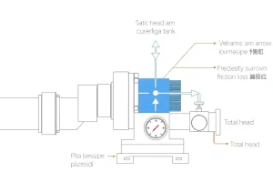
K‑factors and equivalent length are two complementary methods for expressing the pressure (or head) drop that occurs when a fluid negotiates a valve, elbow, tee, reducer or any other fitting. The loss originates from turbulence, flow separation and vena‑contracta effects that convert useful kinetic energy into heat. In pump‑system design the sum of these losses determines the required total dynamic head (TDH), the pump size, motor power, and ultimately the operating cost of the plant.
Under‑estimating fitting losses can cause a pump to run at higher suction lift, increase the risk of cavitation, produce excessive vibration, or even lead to premature seal failure. Conversely, over‑estimating losses may result in an oversized pump that wastes electricity and capital expense.
The Method — Derivation and Variants
The starting point is Bernoulli’s equation with an added loss term:
P_1/rho g + v_1²/(2g) + z_1 = P_2/rho g + v_2²/(2g) + z_2 + h_f
For a fitting of constant diameter and negligible elevation change, v_1≈v_2=v, giving:
h_f = Delta P/(rho g)
Experimental data show that the pressure drop across most fittings can be expressed as:
Delta P = K·rho v²/2
Dividing by rho g yields the classic head‑loss equation shown in the Key Facts Box.
US‑customary form (ft, ft/s):
h_f (ft) = K·v²/(2·32.174)
SI form (m, m/s):
h_f (m) = K·v²/(2·9.80665)
When a K‑value is not tabulated, the fitting is replaced by an equivalent length L_eq that would produce the same loss in a straight pipe. Using the Darcy‑Weisbach friction loss for a straight pipe:
h_f = f·(L/D)·v²/(2g)
Setting L = L_eq and solving for L_eq gives the conversion:
L_eq = K·D/f
Thus the same K‑value can be translated into an extra length of pipe, provided the same Darcy friction factor f applies to the entire network.
Worked Example
Scenario: A water‑cooling loop carries 500 gpm (31.5 L/s) through a 4‑in (0.102 m) schedule 40 steel pipe. The line contains a fully‑open globe valve (K=10), a standard 90° elbow (K=0.9) and a fully‑open gate valve (K=0.15). Straight‑pipe length (excluding fittings) is 150 ft (45.7 m). Determine the total head loss using both the K‑factor approach and the equivalent‑length approach.
- Calculate mean velocity.
US: v = Q / A = 500 gpm / (π·(4 in/12)²/4) ≈ 23.5 ft/s.
SI: v = 31.5 L/s / (π·(0.102 m)²/4) ≈ 1.22 m/s. - Head loss for each fitting (K‑factor method).
US:
Globe valve: 10·23.5²/(2·32.174) ≈ 85.5 ft.
90° elbow: 0.9·23.5²/(2·32.174) ≈ 7.7 ft.
Gate valve: 0.15·23.5²/(2·32.174) ≈ 1.3 ft.
SI:
Globe valve: 10·1.22²/(2·9.80665) ≈ 0.76 m.
Elbow: 0.9·1.22²/(2·9.80665) ≈ 0.07 m.
Gate valve: 0.15·1.22²/(2·9.80665) ≈ 0.01 m. - Pipe friction loss.Assume turbulent flow, Darcy friction factor f = 0.018 (new steel, Re≈1.1×10⁵).
US: h_f(pipe) = f·L/D·v²/(2g) = 0.018·150/0.333·23.5²/(2·32.174) ≈ 41.2 ft.
SI: h_f(pipe) = 0.018·45.7/0.102·1.22²/(2·9.80665) ≈ 12.5 m. - Total head loss (K‑factor method).
US: 85.5 + 7.7 + 1.3 + 41.2 ≈ 135.7 ft.
SI: 0.76 + 0.07 + 0.01 + 12.5 ≈ 13.34 m. - Equivalent‑length method.Typical L_eq/D values: globe valve ≈ 30 D, elbow ≈ 3 D, gate valve ≈ 0.5 D. For D = 4 in = 0.333 ft, L_eq,total = (30+3+0.5)·0.333 ≈ 11.2 ft. Add to straight length → 161.2 ft. Using the same f and velocity gives h_f ≈ 144 ft, close to the summed‑K result.
The example demonstrates that a single globe valve can dominate the total loss, reinforcing the importance of accurate K‑values.
Calculator
For quick verification, use an online total‑dynamic‑head tool such as PumpCalcs – Total Dynamic Head Calculator.
Reference Values & Typical Ranges
| Fitting | K (water, Re ≈ 10⁵‑10⁶) | L_eq/D (equivalent length) |
|---|---|---|
| Globe valve (fully open) | 10‑12 | 30‑35 |
| Gate valve (fully open) | 0.10‑0.20 | 0.5‑1.0 |
| Ball valve (full open) | 0.05‑0.15 | 0.25‑0.5 |
| 90° standard elbow | 0.8‑1.2 | 2.5‑3.5 |
| Long‑radius elbow (R = 2D) | 0.3‑0.5 | 1.2‑1.5 |
| Tee, straight‑through | 0.6‑0.8 | 2.0‑2.5 |
| Tee, branched | 1.8‑2.5 | 6‑8 |
Values are compiled from ASME B31.3 Appendix C, Crane Technical Paper 410, and CIBSE Guide C.
Application Guidance
- System‑level sizing: Use equivalent length when a single Darcy friction factor will be applied to all straight‑pipe sections; this keeps the iterative pipe‑sizing process simple.
- Component‑level analysis: Prefer K‑factors for individual valve or fitting selection, especially when the fitting operates at a non‑standard flow coefficient (C_v).
- Viscosity and Reynolds‑number effects: In turbulent flow K‑values are relatively insensitive to viscosity, but for laminar regimes (Re < 2000) a Reynolds‑number correction factor is required (often 0.8·(Re/2000)^0.5).
- Field adjustments: Add 10‑15 % to tabulated K‑values for dirty, corroded, or poorly aligned fittings.
- Software integration: CFD packages provide pressure‑drop results directly; for hand calculations the K‑factor method remains the industry‑standard quick‑check.
Common Mistakes, Limits & Safety Notes
- Mixing US and SI units within a single calculation – keep g, v and K in consistent units.
- Applying a water‑based K‑value to oil, steam or highly viscous fluids without correction – density and compressibility alter the turbulence pattern.
- Using equivalent length for fittings that change pipe diameter (reducers, expanders); the conversion assumes constant D.
- Neglecting Reynolds‑number dependence for low‑flow conditions; K can be up to 40 % lower in laminar flow.
- Double‑counting losses – do not add both a K‑based loss and its equivalent length for the same fitting.
- Assuming a single friction factor for a network that contains different materials or roughness values.
- Overlooking cavitation risk in high‑head valves; excessive loss raises suction NPSH requirements.
- Safety consequence: Under‑estimating total loss can force the pump to operate near its shut‑off head, increasing seal wear and the chance of pipe rupture.
FAQ
How do I choose between using a K‑factor and an equivalent length?
Use a K‑factor when you have the specific fitting data and need a quick, component‑level loss. Use equivalent length when you are performing a system‑wide Darcy‑Weisbach calculation and want to treat all losses as additional pipe length.
Can I apply water‑based K‑values to oil or steam?
Not directly. Viscosity, density and compressibility affect turbulence. Apply a correction factor based on Reynolds number or use manufacturer‑provided K‑values for the specific fluid.
What is the typical uncertainty associated with tabulated K‑values?
For turbulent water flow the uncertainty is usually ±10 % to ±15 %, increasing to ±30 % for low‑Re laminar conditions or when fittings are fouled.
How does pipe roughness influence the equivalent‑length method?
Roughness changes the Darcy friction factor f. Since L_eq = K·D/f, an inaccurate f will mis‑represent the equivalent length. Use the appropriate f for the material and flow regime.
Why does the globe valve dominate the total head loss in many systems?
A globe valve forces the fluid through a narrow seat and a restricted flow path, creating a high turbulence level and a large K‑value (10‑12), which often exceeds the friction loss of many feet of straight pipe.
Is it acceptable to add the equivalent lengths of all fittings to the pipe length and then apply a single friction factor?
Yes, this is the standard practice when the same f applies to the entire network. Ensure that no fitting changes the pipe diameter, as the conversion assumes constant D.
What correction is needed for K‑values in laminar flow?
A common correction multiplies the turbulent‑flow K by 0.8·(Re/2000)^0.5, reducing the loss as the flow becomes more orderly.
How do I account for high‑temperature fluids that change density?
Re‑calculate the fluid density at operating temperature and use it in the pressure‑drop relationship ΔP = K·ρ·v²/2. The K‑value itself is usually unchanged for turbulent flow.
Leave a Reply