
Short Answer
Key Formula / Key Facts Box
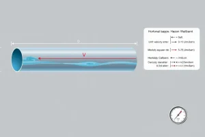
Hazen‑Williams Friction‑Loss Equation (US Units)
[h_f = 10.67 frac{L,Q^{1.852}}{C^{1.852} D^{4.87}}]
Hazen‑Williams Friction‑Loss Equation (SI Units)
[h_f = 4.727 frac{L,Q^{1.852}}{C^{1.852} D^{4.87}}]
| Symbol | Meaning | US Unit | SI Unit |
|---|---|---|---|
| h_f | Head loss due to friction | feet (ft) | meters (m) |
| L | Pipe length | feet (ft) | meters (m) |
| Q | Volumetric flow rate | gallons per minute (gpm) | liters per second (L/s) |
| D | Inside pipe diameter | inches (in) | millimeters (mm) |
| C | Hazen‑Williams roughness coefficient | – | – |
In plain English: friction loss rises with pipe length and flow rate, but falls sharply as pipe diameter or material smoothness (higher C) increase.
Overview — What It Is and Why It Matters
The Hazen‑Williams C value is an empirical, dimension‑less number that characterises the relative smoothness of a pipe’s interior surface when water (at approximately 60 °F or 15.6 °C) flows turbulently. Developed for municipal water distribution, the C value replaces the more fundamental Darcy‑Weisbach friction factor with a single coefficient that captures surface texture, age‑related scaling, and manufacturing tolerances.
Accurate C values are crucial because friction loss typically dominates the total dynamic head (TDH) in low‑pressure, high‑flow water‑service networks. An error of 20 % in C can translate into a comparable error in pump sizing, energy consumption, and compliance with fire‑flow or pressure‑regulation codes.
The Method — Derivation and Variants
The original Hazen‑Williams relationship emerged from extensive laboratory testing of water flowing through a variety of pipe materials. The data showed that, for turbulent flow (Re > 10 000), head loss varied roughly as the 1.852 power of flow rate and the –4.87 power of pipe diameter. By fitting these exponents to the experimental data, the empirical equation was obtained.
US‑customary form:
[h_f = K_{US},frac{L,Q^{1.852}}{C^{1.852} D^{4.87}}] where (K_{US}=10.67).
Metric form:
[h_f = K_{SI},frac{L,Q^{1.852}}{C^{1.852} D^{4.87}}] where (K_{SI}=4.727). The SI constant incorporates unit‑conversion factors between gpm → L/s, inches → mm, and feet → m.
- The exponent 1.852 reflects the nonlinear increase of turbulent loss with flow.
- The exponent 4.87 captures the strong inverse relationship with pipe diameter.
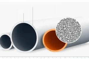
- C is dimensionless; higher values indicate smoother interiors (e.g., new PVC), lower values indicate rougher materials (e.g., aged cast iron).
When water temperature deviates markedly from 60 °F, a temperature correction factor (typically 0.85–1.15) may be applied, but most design work uses the base C value.
Worked Example
Example 1 – US Units (Schedule 40 PVC)
Design a domestic water line that delivers 250 gpm through 300 ft of PVC pipe with an inside diameter of 2.027 in. The manufacturer lists C = 150 for new PVC. Compute the friction loss.
- Insert values into the US‑customary equation.
- Calculate each term (using a calculator):
• (Q^{1.852}=250^{1.852}approx 4.48times10^{3})
• (C^{1.852}=150^{1.852}approx 1.92times10^{3})
• (D^{4.87}=2.027^{4.87}approx 35.2) - Apply the formula:
[h_f = 10.67timesfrac{300times4.48times10^{3}}{1.92times10^{3}times35.2}approx 215text{ ft}]
Result: friction loss ≈ 215 ft of water (≈ 655 psi), indicating the need for a larger diameter or reduced flow to meet typical residential pressure limits.
Example 2 – SI Units (Ductile‑Iron)
A municipal branch requires 8 L/s through 150 m of ductile‑iron pipe (ID = 150 mm). New ductile‑iron C = 130. Compute head loss.
- Insert into the SI form.
- Calculate:
• (Q^{1.852}=8^{1.852}approx 55.0)
• (C^{1.852}=130^{1.852}approx 1.55times10^{3})
• (D^{4.87}=150^{4.87}approx 1.03times10^{6}) (mm⁴·⁸⁷) - Convert diameter to meters for the constant (150 mm = 0.150 m) and apply:
[h_f = 4.727timesfrac{150times55.0}{1.55times10^{3}times0.150^{4.87}}approx 9.8text{ m}]
Result: friction loss ≈ 9.8 m of water (≈ 32 ft), which is acceptable for most pressure‑regulation schemes.
Calculator
For quick computations, use the online Hazen‑Williams calculator: http://pumpcalcs.com/calculators/hazen-williams.
Reference Values & Typical Ranges
| Pipe Material | Typical C Value (New) | Typical C Value (Aged) |
|---|---|---|
| PVC (Schedule 40) | 150 | 130‑140 |
| CPVC | 150 | 135‑145 |
| Ductile‑Iron | 130 | 100‑115 |
| Cast Iron | 130 | 80‑100 |
| Galvanised Steel | 120 | 90‑110 |
| Stainless Steel | 120‑130 | 110‑120 |
| Concrete (smooth) | 140 | 115‑130 |
Values are drawn from AWWA M36, ASTM D1785, and industry handbooks. Age‑related reduction is typical after 10‑15 years of service.
Application Guidance
- Use the highest applicable C value for new installations; apply a reduction factor for known scaling or corrosion.
- When designing for fire‑flow, adopt conservative (lower) C values to avoid under‑estimating head loss.
- For long‑run mains (> 500 ft), small errors in C compound; consider a sensitivity analysis.
- Combine Hazen‑Williams with Darcy‑Weisbach for high‑temperature or high‑viscosity fluids where the original empirical basis is invalid.
- Document the source of each C value (manufacturer data sheet, code reference) for future maintenance.
Common Mistakes, Limits & Safety Notes
- Mixing US and SI units in the same calculation – always keep the constant (10.67 or 4.727) consistent with the unit system.
- Applying Hazen‑Williams to non‑water fluids or to water far from 60 °F without a temperature correction.
- Using a single C value for a pipe network that contains multiple materials or varying ages; segment the system.
- Neglecting minor‑loss coefficients (fittings, valves) which can be comparable to friction loss in short runs.
- Assuming the Hazen‑Williams equation is valid for laminar flow (Re < 2000); in that regime Darcy‑Weisbach should be used.
- Over‑reliance on rounded C tables – small differences (e.g., 150 vs 145) can affect pump selection in marginal designs.
FAQ
How do I choose the correct C value for aged pipe?
Start with the material’s new‑pipe C value, then apply a reduction factor based on visual inspection, water quality data, or manufacturer‑provided aging curves—typically 10‑30 % lower after 10 years.
Can the Hazen‑Williams equation be used for hot water?
Only with a temperature correction factor. The base C values assume 60 °F; for temperatures above 80 °F, multiply C by 0.85‑0.95 to account for viscosity changes.
What is the impact of fittings on Hazen‑Williams calculations?
Fittings are accounted for with equivalent length or minor‑loss coefficients, which are added to the actual pipe length before applying the Hazen‑Williams equation.
Is Hazen‑Williams appropriate for non‑water fluids?
No. The equation is empirical for water at moderate temperatures. For oils, refrigerants, or high‑viscosity liquids, use Darcy‑Weisbach with appropriate fluid properties.
Why does the exponent on flow rate differ from the Darcy‑Weisbach exponent of 2?
Hazen‑Williams is a curve‑fit to experimental data; the 1.852 exponent provides a better fit for turbulent water flow in typical pipe materials than the theoretical exponent of 2.
How sensitive is pump size to errors in C value?
A 10 % error in C can produce roughly a 5‑7 % error in estimated head loss, which may lead to selecting a pump that is oversized by 5‑10 % or undersized, affecting energy use and reliability.
Do PVC and CPVC have the same C value?
Both are generally assigned a C of 150 when new, but CPVC may retain a slightly higher value over time due to better resistance to scaling.
When should I switch to Darcy‑Weisbach instead of Hazen‑Williams?
Use Darcy‑Weisbach when dealing with temperatures far from 60 °F, non‑water fluids, laminar flow, or when high‑precision analysis is required.



Leave a Reply