Short Answer
Key Formula / Key Facts Box
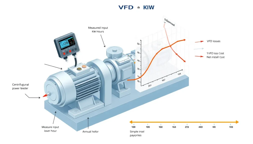
Governing payback equation. For measured electrical input power at each operating state:
Pin,3φ = √3 × VLL × IL × PF ÷ 1000 (kW)
Ebase = Σ(Pbase,i × ti); EVFD = Σ(PVFD,i × ti)
Annual savings = (Ebase - EVFD) × energy price

Simple payback = (installed cost - incentives) ÷ annual savings
| Symbol | Meaning | US unit | SI unit |
|---|---|---|---|
Pin,3φ |
Real three-phase electrical input power | kW | kW |
VLL |
Line-to-line voltage | V | V |
IL |
Line current | A | A |
PF |
Power factor, dimensionless | — | — |
Pbase,i |
Measured baseline input power in interval i | kW | kW |
PVFD,i |
Projected or measured post-VFD input power in interval i | kW | kW |
ti |
Operating hours in interval i | h/yr | h/yr |
| Energy price | Electricity cost | $/kWh | currency/kWh |
Plain-English restatement: Multiply measured kilowatts by hours at each duty point, subtract the VFD-case kilowatt-hours, multiply by the energy price, and divide net project cost by that annual saving.
Overview — What It Is and Why It Matters
How to calculate VFD payback using measured pump input power is a measurement-based economic method for deciding whether a variable frequency drive will recover its installed cost. In this article, measured pump input power means real electrical input power at the motor feeder or drive input, expressed in kilowatts. It is not hydraulic power, not shaft power, and not current alone. That distinction is the scope chosen here because current-only estimates are common screening tools but do not establish real energy use.
VFD savings are frequently overestimated when a nameplate horsepower, a running current, or a simple cube-law assumption is used without a measured baseline. A pump that is throttled by a control valve may show a large pressure drop, but the actual electrical saving depends on the annual flow profile, static head, pump efficiency, motor efficiency, VFD losses, and hours at each operating state. Chelan PUD notes that VFD savings on irrigation pumps can be small or negligible unless the existing control method wastes energy and flow varies significantly. Industrial Monitor Direct makes the same point more broadly: current and rated current cannot quantify savings; real input power integrated across the operating profile is the number that matters.
The method matters because payback is a capital decision. A project with a two-year simple payback is usually easy to justify; a project with a twelve-year payback may fail a capital screen even if it saves some energy. Measured input power also creates a defensible measurement and verification boundary for utility incentive programs and for post-retrofit checks, as shown in Save on Energy sample M&V plans.
The Method — Derivation and Variants
The derivation starts with electrical power. For a balanced three-phase motor, real input power is Pin = √3 × VLL × IL × PF in watts. Dividing by 1000 gives kW. For a single-phase motor, Pin = V × I × PF ÷ 1000 kW. If a power analyzer or permanent meter reads kW directly, that reading is preferred because it avoids errors in voltage, current, and power factor. Current alone is insufficient because the same current can occur at different voltage and power factor conditions.
Next, build an annual energy baseline: Ebase = Σ(Pbase,i × ti). Each interval should represent a real operating state, such as full flow, 75% flow, 60% flow, and 50% flow. The hours must come from logs, historian trends, runtime counters, or a representative metering campaign. A single spot reading may establish one duty point but cannot define annual energy.
Then estimate the VFD-case power at the same measurement boundary. The strongest method is a controlled before-and-after trial with measured kW, flow, and pressure. The next strongest is a pump-and-system-curve model using the measured baseline power to calibrate the existing point. A common screening variant uses affinity-law scaling: Q2/Q1 ≈ N2/N1, H2/H1 ≈ (N2/N1)2, and shaft power P2/P1 ≈ (N2/N1)3. The cube relationship applies best to friction-dominated systems and similar efficiency; it is not an automatic savings formula for high-static-head systems. Include VFD losses, typically 2% to 5%, and use motor efficiency at the actual speed and load.
| Form | US customary | SI |
|---|---|---|
| Electrical input power | kW = √3 × V × A × PF ÷ 1000 |
kW = √3 × V × A × PF ÷ 1000 |
| Energy | kWh = kW × h |
kWh = kW × h |
| Hydraulic power, if needed | hp = Q(gpm) × H(ft) × SG ÷ 3960 |
kW = ρ × g × Q(m3/s) × H(m) ÷ 1000 |
Variants differ mainly in data quality. Direct metering with a power logger is best for the baseline. Short-term logging plus a validated system model is acceptable when annual data are unavailable. Calculated kW from simultaneous voltage, current, and power factor is acceptable if the instrument and power factor are reliable. Nameplate-only estimates should be treated as screening guesses, not payback calculations. Simple payback is appropriate for screening; life-cycle cost or net present value is better for large projects because simple payback ignores energy-price escalation and time value of money.
Worked Example
US customary example. A 100 hp constant-speed pump is throttled to meet variable demand. A three-phase power analyzer logs 480 V, 88 A, and 0.86 power factor at the dominant duty point. Calculate measured input power: P = √3 × 480 × 88 × 0.86 ÷ 1000 = 62.9 kW. Assume the annual duty profile averages 62.9 kW for 6,000 h/yr, so baseline energy is 62.9 × 6,000 = 377,400 kWh/yr. At $0.12/kWh, baseline cost is $45,288/yr. A validated system model projects a VFD average of 48.5 kW, saving 14.4 kW. Annual saving is 14.4 × 6,000 = 86,400 kWh/yr, or 86,400 × 0.12 = $10,368/yr. If installed cost is $35,000 and the utility incentive is $5,000, net cost is $30,000. Simple payback is 30,000 ÷ 10,368 = 2.9 years. If high static head limits speed reduction, use a higher VFD-case kW and the payback lengthens.
SI example. A 75 kW motor-pump set is measured at 400 V, 105 A, and 0.88 power factor. Input power is √3 × 400 × 105 × 0.88 ÷ 1000 = 64.0 kW. The pump runs 5,500 h/yr at this measured profile. Baseline energy is 64.0 × 5,500 = 352,000 kWh/yr. A VFD trial projects 50.0 kW average, saving 14.0 kW. Annual saving is 14.0 × 5,500 = 77,000 kWh/yr. At €0.18/kWh, annual cost saving is €13,860. With net installed cost of €32,000 after incentives, simple payback is 32,000 ÷ 13,860 = 2.3 years. Always compare baseline and VFD power at the same boundary: motor feeder, drive input, or drive output plus drive loss.
Calculator
For hydraulic inputs and system-curve checks, use the PumpCalcs Total Dynamic Head calculator at pumpcalcs.com/calculators/total-dynamic-head/. Pair the head calculation with measured kW and hours in a spreadsheet to compute annual energy and simple payback. For commercial VFD screening, the Xylem VSD Payback Tool is also cited in the references.
Reference Values & Typical Ranges
| Item | Typical range or rule of thumb | Engineering note |
|---|---|---|
| VFD efficiency | 95% to 98% | Include drive losses in the VFD-case kWh; Xylem payback tool accounts for drive and motor data. |
| Motor efficiency | 85% to 95% | Depends on size, loading, and age; use actual data when available. |
| Power factor | 0.75 to 0.90 at partial load | Must be measured; current-only estimates are not defensible. |
| Attractive simple payback | 1 to 5 years | Common screening range for throttled pumps with variable duty; verify project-specific costs. |
| Small pump threshold | Below about 5 hp | Often not economic for VFD retrofit without other benefits, per Sustainable Engineering guidance. |
| Lightly throttled valve | Less than 20% closed | Little added head loss to recover; savings may be small. |
| Static head fraction | About 30% of total design head if unknown | Xylem suggests this default for screening; higher static head reduces VFD savings. |
These values are screening aids, not guarantees. Chelan PUD emphasizes that savings depend on the existing control method, pressure setpoint, annual hours, flow profile, and pump curve. Industrial Monitor Direct recommends detailed analysis when variable flow occurs outside 80% to 110% of best-efficiency-point flow for more than half of operating time, with significant time in the 50% to 70% range. Treat such thresholds as proposal screening assumptions and verify with the actual pump curve.
Application Guidance
In real systems, VFD savings are strongest when the existing pump runs at constant speed and the flow is throttled, bypassed, or otherwise wasted. A pressure-reducing valve creates an artificial head loss; a VFD can reduce speed and remove that loss, but only if the system still requires the lower head. In high-static-head systems, such as deep-well or elevation-dominated pumping, the pump must still overcome static lift even at low flow, so speed reduction is limited and the cube law overstates savings. Measure static head and compare it with total dynamic head before promising payback.
Use the measured baseline to select the VFD and motor package. Confirm that the motor is inverter-duty or suitable for variable-speed operation, check cable length and carrier frequency limits, evaluate harmonics if the drive is large relative to the supply, and verify minimum pump speed and minimum flow. For pumps with flat curves, pressure control may be stable; for steep curves, flow or pressure setpoints need careful tuning. Field judgment should adjust the annual hours, add VFD and motor losses, account for reduced pump efficiency away from the best efficiency point, and include maintenance or reliability value only if it is separately justified.
A defensible study usually includes one week or more of power logging, simultaneous flow and pressure readings at representative states, a written duty profile, and a post-installation verification plan. Utility incentives can change the payback materially, so include them in net installed cost. If the measured power data show a lightly loaded motor with high power factor and little throttling loss, the project may have a long payback even if the pump is large.
Common Mistakes, Limits & Safety Notes
- Using running current or nameplate current as if it were power. Current does not give kW without voltage and power factor.
- Ignoring power factor, especially at partial load where it can fall significantly.
- Mixing hydraulic power, shaft power, and electrical input power in the same payback calculation.
- Using a single spot measurement to represent an entire year instead of building a duty profile.
- Applying the cube law to high-static-head systems where speed reduction is limited.
- Forgetting VFD losses, motor efficiency changes, and pump efficiency changes at reduced speed.
- Comparing baseline motor-feeder kW with VFD-output kW without adding drive losses.
- Ignoring incentives, installation cost, engineering cost, and electrical upgrade cost in net project cost.
- Treating simple payback as a full financial analysis; it ignores energy-price escalation and time value of money.
- Taking electrical measurements without qualified personnel, lockout/tagout, arc-flash assessment, and appropriate PPE. Safety consequences include shock, arc flash, and unexpected pump start.
FAQ
How do I measure pump input power for a VFD payback study?
Use a three-phase power analyzer or permanent meter to log real kW at the motor feeder or VFD input. Record voltage, current, power factor, flow, and pressure simultaneously at each operating state. A current-only reading is not enough because kW depends on voltage and power factor; integrate the logged kW over a representative annual duty profile.
Can I calculate VFD savings from running current alone?
No. Running current shows loading at one instant but does not give real power without voltage and power factor. It also says nothing about annual hours or hydraulic useful output. Use current for screening only; base payback on measured kW or a metered kWh baseline, then compare with a projected or measured VFD-case power at the same boundary.
Why does high static head reduce VFD payback?
In a high-static-head system, the pump must still produce most of the same head even when flow falls. Speed reduction is therefore limited, so power does not fall as much as the cube law predicts. Measure static head and total dynamic head, then use a system-curve model or trial rather than applying a generic cube-law saving.
What annual operating hours should I use in the payback formula?
Use hours at each actual flow and power condition, not just total annual runtime. A pump that runs 6,000 hours per year may spend only part of that time throttled. Build bins from historian data, operator logs, or a representative metering period. If only total hours are available, document that uncertainty and run low, base, and high cases.
Should VFD losses be included in the savings calculation?
Yes. A VFD typically has 95% to 98% efficiency, and additional losses occur in cables, filters, and the motor at reduced speed. Compare baseline and post-retrofit power at the same measurement boundary. If baselining at the motor feeder, add drive losses when projecting VFD-input kW so the payback is not overstated.
What is a good simple payback for a pump VFD?
Many facilities screen projects at one to five years, but the threshold depends on capital policy, energy price, incentives, and non-energy benefits. A two-year payback is usually attractive; a ten-year payback may still be justified by reliability or process control but should be evaluated with life-cycle cost rather than simple payback alone.
What if I do not have a pump performance curve?
Use field measurements as a substitute: simultaneous kW, flow, pump discharge pressure, pressure downstream of the throttle or bypass, and hours at each state. A controlled temporary speed trial can provide direct before-and-after data. If curves are unavailable, avoid claiming precise savings from a cube-law calculation; present a range with clearly stated assumptions.
How do utility incentives affect VFD payback?
Incentives reduce net installed cost and therefore shorten simple payback. Include the expected incentive in the numerator only after confirming eligibility and measurement requirements. Keep the gross installed cost visible for transparency, and follow the utility M&V plan because baseline and post-retrofit metering rules can affect the approved savings.
Leave a Reply