
Short Answer
Key Formula / Key Facts Box
Darcy–Weisbach head‑loss equation
[h_f = f frac{L}{D}frac{V^{2}}{2g}]
| Symbol | Meaning | US Unit | SI Unit |
|---|---|---|---|
| h_f | Frictional head loss | ft | m |
| f | Darcy friction factor (dimensionless) | — | — |
| L | Pipe length | ft | m |
| D | Inside pipe diameter | in or ft | mm or m |
| V | Mean flow velocity | ft/s | m/s |
| g | Acceleration due to gravity | 32.174 ft/s² | 9.80665 m/s² |
In plain English: the head loss equals the friction factor times the length‑to‑diameter ratio multiplied by the kinetic‑energy term V²/2g.
Overview — What It Is and Why It Matters
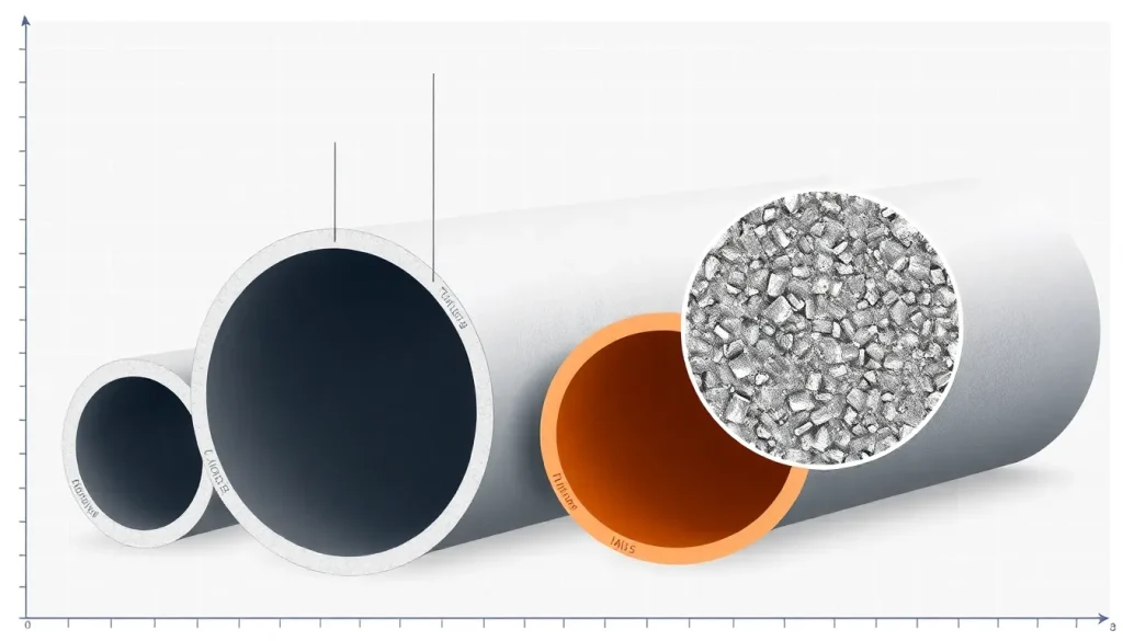
Pipe roughness quantifies the microscopic irregularities on the interior surface of a conduit. These asperities disrupt the laminar sub‑layer, increasing turbulence and therefore the frictional losses that a pump must overcome. Engineers use roughness (ε) together with the Reynolds number to determine the Darcy friction factor via the Colebrook‑White or Moody chart. Selecting an inappropriate ε value can lead to under‑ or over‑sized pumps, excess energy consumption, premature wear, and even system failure.
The Method — Derivation and Variants
The Darcy–Weisbach equation is derived from the mechanical energy balance for a steady, incompressible flow. The friction factor f is obtained from empirical relationships that capture the transition from smooth‑pipe (laminar) to rough‑pipe (turbulent) regimes. Two common forms are:
- Colebrook‑White equation (implicit) – valid for 4 000 < Re < 10⁸:
[frac{1}{sqrt{f}} = -2log_{10}!left(frac{varepsilon/D}{3.7}+frac{2.51}{mathrm{Re}sqrt{f}}right)]
- Swamee‑Jain explicit approximation – useful for hand calculations:
[f = 0.25left[log_{10}!left(frac{varepsilon/D}{3.7}+frac{5.74}{mathrm{Re}^{0.9}}right)right]^{-2}]
In the US customary system the same equations use feet, inches, and the constant 32.174 ft/s² for g; in SI they use meters and 9.80665 m/s². The roughness ε is expressed either in millimetres (mm) or mils (1 mil = 0.001 in). The choice of variant depends on required accuracy and available computational tools.
Worked Example
Example 1 – SI Units (Carbon Steel pipe)
Design a water‑distribution loop that transports 0.12 m³/s through a 150 m length of Schedule 40 steel pipe (DN 150, ID ≈ 0.145 m). Determine the head loss using the Swamee‑Jain equation. Assume ε = 0.045 mm for commercial carbon steel and water at 20 °C (ν ≈ 1.003 × 10⁻⁶ m²/s).
- Compute velocity:
V = Q/A = 0.12 / (π·0.145²/4) ≈ 7.30 m/s. - Reynolds number: Re = V·D/ν ≈ 7.30·0.145/1.003e‑6 ≈ 1.05 × 10⁶ (turbulent).
- Relative roughness: ε/D = 0.045 mm / 145 mm ≈ 3.10 × 10⁻⁴.
- Swamee‑Jain friction factor:
f = 0.25 [log₁₀( (ε/D)/3.7 + 5.74/Re⁰·⁹ )]⁻²
≈ 0.25 [log₁₀(8.38e‑5 + 5.74/(1.05e⁶)⁰·⁹ )]⁻²
≈ 0.0195. - Head loss: h_f = f·L/D·V²/(2g)
≈ 0.0195·150/0.145·7.30²/(2·9.80665)
≈ 7.2 m.
Example 2 – US Customary Units (PVC pipe)
Move 250 gpm of water through 500 ft of 4‑in ID PVC (ε ≈ 0.0015 mm ≈ 0.000059 in). Use the Colebrook‑White equation (solved iteratively).
- Convert flow: Q = 250 gpm = 0.557 ft³/s.
- Area: A = π·(4 in/12)²/4 ≈ 0.349 ft² → V = Q/A ≈ 1.60 ft/s.
- Reynolds: ν (water at 68 °F) ≈ 1.12 × 10⁻⁵ ft²/s → Re = V·D/ν ≈ 1.60·0.333/1.12e‑5 ≈ 4.8 × 10⁴.
- Relative roughness: ε/D = 0.000059 / 0.333 ≈ 1.77 × 10⁻⁴.
- Iterate Colebrook‑White; after 3 iterations f ≈ 0.023.
- Head loss: h_f = f·L/D·V²/(2g)
= 0.023·500/0.333·1.60²/(2·32.174)
≈ 0.84 ft.
Calculator
For quick verification, use an online Darcy–Weisbach head‑loss calculator: http://pumpcalcs.com/calculators/total-dynamic-head/
Reference Values & Typical Ranges
| Material | Typical Roughness ε (mm) | Typical Roughness ε (mil) | Notes |
|---|---|---|---|
| Commercial Carbon Steel (new) | 0.045 | 1.8 | ISO 1043‑1, smooth after manufacturing. |
| Carbon Steel (corroded) | 0.150 – 0.300 | 6 – 12 | Scale and pitting increase ε. |
| Stainless Steel (AISI 304) | 0.015 | 0.6 | Generally smoother than carbon steel. |
| Galvanized Steel | 0.050 | 2.0 | Coating adds modest roughness. |
| Copper (drawn) | 0.0015 | 0.06 | Very smooth; often treated as smooth pipe. |
| PVC (Schedule 40) | 0.0015 | 0.06 | Manufacturing tolerances keep ε low. |
| HDPE (SDR 11) | 0.0015 | 0.06 | Extruded, smooth wall. |
| Concrete (cast‑in‑place) | 0.300 – 1.500 | 12 – 60 | Surface finish dominates. |
| Glass | 0.001 | 0.04 | Effectively smooth. |
Values are taken from ISO 1043‑1, ASME B36.10, and the Crane Technical Paper No. 410. When a material’s condition is uncertain, adopt the higher end of the range to provide a conservative design.
Application Guidance
- Always use the *inside* diameter for D; nominal pipe sizes are misleading.
- For newly installed commercial steel, treat ε ≈ 0.045 mm unless a rough‑finished surface is specified.
- If the pipe will be exposed to corrosion, scale, or abrasive slurries, increase ε by 50‑100 % to capture future degradation.
- When mixing materials (e.g., steel to PVC), calculate head loss for each segment separately and sum the results.
- In high‑Re regimes (Re > 10⁵) the friction factor becomes insensitive to Reynolds number; roughness dominates.
- For low‑Re laminar flow (Re < 2 300) roughness is irrelevant; f = 64/Re.
Common Mistakes, Limits & Safety Notes
- Using nominal diameter instead of ID. This can underestimate head loss by up to 15 %.
- Confusing ε (mm) with ε/D (dimensionless). Plug the raw roughness into the Colebrook‑White equation without forming the ratio yields nonsense.
- Mixing US and SI units in the same calculation. Always convert before substitution; g, ν, and ε must share a consistent system.
- Applying the Darcy‑Weisbach equation to extremely low‑pressure systems without checking laminar assumptions. In laminar flow the simpler Hagen–Poiseuille equation is more accurate.
- Neglecting pipe aging. Roughness increases with time; designs that ignore this may suffer higher pump energy costs.
- Using the Hazen‑Williams C‑factor as a surrogate for ε. The two are not interchangeable; Hazen‑Williams is empirical for water at 60 °F.
- Ignoring temperature effects on viscosity. Water viscosity changes ~2 % per 10 °F; for precise design, update ν accordingly.
- Over‑reliance on the Swamee‑Jain approximation near the transition region (Re ≈ 4 000‑10 000). An iterative Colebrook solution is recommended there.
FAQ
How do I decide whether to use the Colebrook‑White or Swamee‑Jain equation?
Use Colebrook‑White when high accuracy is required, especially near the transition Reynolds range (4 000‑10 000) or when the pipe roughness is large. Swamee‑Jain provides a quick explicit estimate with <5 % error for fully turbulent flow.
Can I treat PVC as a smooth pipe and ignore roughness?
PVC has a very low roughness (≈0.0015 mm) and can be approximated as smooth for most designs, but for long runs or high‑velocity applications include the nominal ε to avoid under‑predicting head loss.
What roughness value should I use for aged steel pipe that may have scale?
Increase the nominal 0.045 mm value by 50‑100 % depending on visual inspection or corrosion reports; a conservative choice is 0.090 mm (≈3.5 mil).
Is the Hazen‑Williams C‑factor a substitute for pipe roughness?
No. Hazen‑Williams is an empirical formula for water at 60 °F; it does not directly provide ε and cannot be used in Darcy‑Weisbach calculations without conversion.
Why does roughness become irrelevant in laminar flow?
In laminar flow (Re < 2 300) the velocity profile is dominated by viscosity, and the friction factor depends only on Re (f = 64/Re). Surface irregularities are smoothed out by the viscous sub‑layer.
My head‑loss calculation seems too low compared to field data. What could be wrong?
Common culprits include using nominal diameter instead of ID, neglecting fittings and valves, using outdated roughness values, or mixing US and SI units. Verify each input and add equivalent length for accessories.
How does temperature affect pipe roughness?
Temperature changes the material’s expansion but has negligible effect on ε itself. However, water viscosity varies with temperature, altering Reynolds number and therefore the friction factor.
Do I need to consider roughness for gas pipelines?
Yes, but gas viscosity is much lower, leading to higher Reynolds numbers; roughness often dominates. Use the same Darcy‑Weisbach framework with appropriate gas properties.




Leave a Reply